dplyr
# install.packages("dplyr")
library(tidyverse)
This document is based on package version of dplyr:
packageVersion("dplyr")
#> [1] '1.0.6'
1 Why dplyr
When working with data you must:
Figure out what you want to do.
Describe those tasks in the form of a computer program.
Execute the program.
The dplyr package makes these steps fast and easy:
By constraining your options, it helps you think about your data manipulation challenges.
It provides simple “verbs”, functions that correspond to the most common data manipulation tasks, to help you translate your thoughts into code.
It uses efficient backends, so you spend less time waiting for the computer.
dplyr codes usually looks like:
starwars %>%
  select(name, height, species) %>%
  filter(species %in% c('Human', 'Droid')) %>%
  mutate(mean_height = mean(height, na.rm = T)) %>%
  group_by(species) %>%
  mutate(mean_height_by_species = mean(height, na.rm = T)) %>%
  ungroup()
Here we use several dplyr “verbs” (select() filter() mutate()) to operate the “data” starwars step by step, and string them together into a pipeline by %>%. We also finish one “by-group” work by wrapping mutate() with group_by() and ungroup(). This code block looks like working left-to-right, top-to-bottom and you can easily find what is done to the data.
So how dplyr do this?
The code dplyr verbs input and output data frames.
dplyr relies heavily on “non-standard evaluation” so that you don’t need to use
$to refer to columns in the “current” data frame.dplyr solutions tend to use a variety of single purpose verbs.
Multiple dplyr verbs are often strung together into a pipeline by
%>%.All dplyr verbs handle “grouped” data frames so that the code to perform a computation per-group looks very similar to code that works on a whole data frame.
2 Tibble
A tibble, or tbl_df, is a modern reimagining of the data.frame, keeping what time has proven to be effective, and throwing out what is not. Tibbles are data.frames that are lazy and surly: they do less (i.e. they don’t change variable names or types, and don’t do partial matching) and complain more (e.g. when a variable does not exist). This forces you to confront problems earlier, typically leading to cleaner, more expressive code. Tibbles also have an enhanced print() method which makes them easier to use with large datasets containing complex objects.
mtcars %>% class()
#> [1] "data.frame"
mtcars %>% as_tibble() %>% class()
#> [1] "tbl_df"     "tbl"        "data.frame"
You can refer to tibbles chapter in R for data science or vignette("tibble") to find the difference between tibble and data.frame.
Tibble is the central data structure for the set of packages known as the tidyverse, including dplyr, ggplot2, tidyr, and readr.
2.1 Creating tibbles
Create a tibble from an existing object with as_tibble(). This will work for reasonable inputs that are already data.frames, lists, matrices, or tables.
as_tibble(iris)
#> # A tibble: 150 x 5
#>   Sepal.Length Sepal.Width Petal.Length Petal.Width Species
#>          <dbl>       <dbl>        <dbl>       <dbl> <fct>
#> 1          5.1         3.5          1.4         0.2 setosa
#> 2          4.9         3            1.4         0.2 setosa
#> 3          4.7         3.2          1.3         0.2 setosa
#> 4          4.6         3.1          1.5         0.2 setosa
#> # … with 146 more rows
You can also create a new tibble from column vectors with tibble(). tibble() will automatically recycle inputs of length 1, and allows you to refer to variables that you just created, as shown below.
tibble(x = 1:5, y = 1, z = x ^ 2 + y)
#> # A tibble: 5 x 3
#>       x     y     z
#>   <int> <dbl> <dbl>
#> 1     1     1     2
#> 2     2     1     5
#> 3     3     1    10
#> 4     4     1    17
#> # … with 1 more row
You can define a tibble row-by-row with tribble(), short for transposed tibble. tribble() is customised for data entry in code: column headings are defined by formulas (i.e. they start with ~), and entries are separated by commas. This makes it possible to lay out small amounts of data in easy to read form.
tribble(
  ~x, ~y,  ~z,
  "a", 2,  3.6,
  "b", 1,  8.5
)
#> # A tibble: 2 x 3
#>   x         y     z
#>   <chr> <dbl> <dbl>
#> 1 a         2   3.6
#> 2 b         1   8.5
2.2 Display
Tibbles have a refined print method that shows only the first 10 rows (we set it to 4 in this document), and all the columns that fit on screen (by default). This makes it much easier to work with large data. In addition to its name, each column reports its type, a nice feature borrowed from str():
starwars
#> # A tibble: 87 x 14
#>   name     height  mass hair_color skin_color  eye_color birth_year sex   gender
#>   <chr>     <int> <dbl> <chr>      <chr>       <chr>          <dbl> <chr> <chr>
#> 1 Luke Sk…    172    77 blond      fair        blue            19   male  mascu…
#> 2 C-3PO       167    75 <NA>       gold        yellow         112   none  mascu…
#> 3 R2-D2        96    32 <NA>       white, blue red             33   none  mascu…
#> 4 Darth V…    202   136 none       white       yellow          41.9 male  mascu…
#> # … with 83 more rows, and 5 more variables: homeworld <chr>, species <chr>,
#> #   films <list>, vehicles <list>, starships <list>
You can also control the default print behaviour by setting options:
options(tibble.print_max = n, tibble.print_min = m): if more than n rows, print only m rows. Useoptions(tibble.print_min = Inf)to always show all rows.Use
options(tibble.width = Inf)to always print all columns, regardless of the width of the screen.
You can see a complete list of options by looking at the package help with package?tibble.
A final option is to use RStudio’s built-in data viewer to get a scrollable view of the complete dataset. This is also often useful at the end of a long chain of manipulations.
starwars %>% view()2.3 Column data types
Refer to vignette("types"), you can find all kinds of column data type in tibble, common are <lgl> for logical, <int> for integer, <dbl> for double, <chr> for character, <date> for Date and so on.
tibble(x1 = T, x2 = 1L, x3 = 1.5, x4 = 'a', x5 = as.Date('2021-03-10'))
#> # A tibble: 1 x 5
#>   x1       x2    x3 x4    x5
#>   <lgl> <int> <dbl> <chr> <date>
#> 1 TRUE      1   1.5 a     2021-03-10
And sometimes you would find <list> for list (list-columns).
tibble(x = list(1, 2:3))
#> # A tibble: 2 x 1
#>   x
#>   <list>
#> 1 <dbl [1]>
#> 2 <int [2]>

mtcars %>% nest_by(cyl)
#> # A tibble: 3 x 2
#> # Rowwise:  cyl
#>     cyl                data
#>   <dbl> <list<tibble[,10]>>
#> 1     4           [11 × 10]
#> 2     6            [7 × 10]
#> 3     8           [14 × 10]
list-columns might be confusing but sometimes it would be useful in modeling while the input are multi tibbles, you can see more details in vignette("rowwise") and Many models chapter in R for data science. Later we will also meet list-columns with “nest” data while study the package tidyr.
2.4 Column names
The name repair described below is exposed to users via the .name_repair argument of tibble::tibble(), tibble::as_tibble(), readxl::read_excel(), and, eventually other packages in the tidyverse.
Tidyverse deals with a few levels of name repair that are practically useful:
minimal: Thenamesattribute is notNULL. The name of an unnamed element is""(the empty string) and neverNA.unique: No element ofnamesappears more than once. A couple specific names are also forbidden in unique names, such as""(the empty string).- All columns can be accessed by name via
df[["name"]]and, more generally, by quoting with backticks:df$`name`,subset(df, select = `name`), anddplyr::select(df, `name`).
- All columns can be accessed by name via
check_unique: It doesn’t perform any name repair. Instead, an error is raised if the names don’t suit the “unique” criteria.universal: Thenamesare unique and syntactic.- Names work everywhere, without quoting:
df$nameandlm(name1 ~ name2, data = df)anddplyr::select(df, name)all work.
- Names work everywhere, without quoting:
c('a', '', NA) %>% vctrs::vec_as_names(repair = 'minimal')
#> [1] "a" ""  ""

c('a', 'b', 'c', 'a') %>% vctrs::vec_as_names(repair = 'unique')
#> New names:
#> * a -> a...1
#> * a -> a...4
#> [1] "a...1" "b"     "c"     "a...4"

c('a', 'b', 'c', 'a') %>% vctrs::vec_as_names(repair = 'check_unique')
#> Error: Names must be unique.
#> x These names are duplicated:
#>   * "a" at locations 1 and 4.

c('(a)', 'b c', '') %>% vctrs::vec_as_names(repair = 'universal')
#> New names:
#> * `(a)` -> .a.
#> * `b c` -> b.c
#> * `` -> ...3
#> [1] ".a."  "b.c"  "...3"
You can see more details in ?vctrs::vec_as_names and Names attribute chapter in Tidyverse design guide.
3 Single table verbs
3.1 Arrange rows by column values: arrange()
arrange() orders the rows of a data frame by the values of selected columns.
starwars %>% arrange(height, mass)
#> # A tibble: 87 x 14
#>   name      height  mass hair_color skin_color eye_color birth_year sex   gender
#>   <chr>      <int> <dbl> <chr>      <chr>      <chr>          <dbl> <chr> <chr>
#> 1 Yoda          66    17 white      green      brown            896 male  mascu…
#> 2 Ratts Ty…     79    15 none       grey, blue unknown           NA male  mascu…
#> 3 Wicket S…     88    20 brown      brown      brown              8 male  mascu…
#> 4 Dud Bolt      94    45 none       blue, grey yellow            NA male  mascu…
#> # … with 83 more rows, and 5 more variables: homeworld <chr>, species <chr>,
#> #   films <list>, vehicles <list>, starships <list>

starwars %>% arrange(desc(height))
#> # A tibble: 87 x 14
#>   name     height  mass hair_color skin_color eye_color birth_year sex   gender
#>   <chr>     <int> <dbl> <chr>      <chr>      <chr>          <dbl> <chr> <chr>
#> 1 Yarael …    264    NA none       white      yellow            NA male  mascul…
#> 2 Tarfful     234   136 brown      brown      blue              NA male  mascul…
#> 3 Lama Su     229    88 none       grey       black             NA male  mascul…
#> 4 Chewbac…    228   112 brown      unknown    blue             200 male  mascul…
#> # … with 83 more rows, and 5 more variables: homeworld <chr>, species <chr>,
#> #   films <list>, vehicles <list>, starships <list>
3.2 Subset distinct/unique rows: distinct()
distinct() select only unique/distinct rows from a data frame.
df <- tibble(
  x = sample(10, 100, rep = TRUE),
  y = sample(10, 100, rep = TRUE)
)
df
#> # A tibble: 100 x 2
#>       x     y
#>   <int> <int>
#> 1     6     8
#> 2     8     2
#> 3     5     8
#> 4     3     6
#> # … with 96 more rows

df %>% nrow()
#> [1] 100

df %>% distinct()
#> # A tibble: 64 x 2
#>       x     y
#>   <int> <int>
#> 1     6     8
#> 2     8     2
#> 3     5     8
#> 4     3     6
#> # … with 60 more rows

df %>% distinct() %>% nrow()
#> [1] 64


df %>% distinct(x)
#> # A tibble: 10 x 1
#>       x
#>   <int>
#> 1     6
#> 2     8
#> 3     5
#> 4     3
#> # … with 6 more rows

df %>% distinct(y)
#> # A tibble: 10 x 1
#>       y
#>   <int>
#> 1     8
#> 2     2
#> 3     6
#> 4     1
#> # … with 6 more rows


df %>% distinct(x, .keep_all = T)
#> # A tibble: 10 x 2
#>       x     y
#>   <int> <int>
#> 1     6     8
#> 2     8     2
#> 3     5     8
#> 4     3     6
#> # … with 6 more rows

df %>% distinct(y, .keep_all = T)
#> # A tibble: 10 x 2
#>       x     y
#>   <int> <int>
#> 1     6     8
#> 2     8     2
#> 3     3     6
#> 4     2     1
#> # … with 6 more rows
3.3 Subset rows using column values: filter()
The filter() function is used to subset a data frame, retaining all rows that satisfy your conditions. To be retained, the row must produce a value of TRUE for all conditions. Note that when a condition evaluates to NA the row will be dropped.
starwars %>%
  filter(hair_color == "none" & eye_color == "black")
#> # A tibble: 9 x 14
#>   name    height  mass hair_color skin_color  eye_color birth_year sex   gender
#>   <chr>    <int> <dbl> <chr>      <chr>       <chr>          <dbl> <chr> <chr>
#> 1 Nien N…    160    68 none       grey        black             NA male  mascul…
#> 2 Gasgano    122    NA none       white, blue black             NA male  mascul…
#> 3 Kit Fi…    196    87 none       green       black             NA male  mascul…
#> 4 Plo Ko…    188    80 none       orange      black             22 male  mascul…
#> # … with 5 more rows, and 5 more variables: homeworld <chr>, species <chr>,
#> #   films <list>, vehicles <list>, starships <list>

starwars %>%
  filter(hair_color == "none" | eye_color == "black")
#> # A tibble: 38 x 14
#>   name     height  mass hair_color skin_color eye_color birth_year sex   gender
#>   <chr>     <int> <dbl> <chr>      <chr>      <chr>          <dbl> <chr> <chr>
#> 1 Darth V…    202   136 none       white      yellow          41.9 male  mascul…
#> 2 Greedo      173    74 <NA>       green      black           44   male  mascul…
#> 3 IG-88       200   140 none       metal      red             15   none  mascul…
#> 4 Bossk       190   113 none       green      red             53   male  mascul…
#> # … with 34 more rows, and 5 more variables: homeworld <chr>, species <chr>,
#> #   films <list>, vehicles <list>, starships <list>
3.4 Subset columns using their names and types: select()
select() select variables in a data frame
starwars %>% select(hair_color, skin_color, eye_color)
#> # A tibble: 87 x 3
#>   hair_color skin_color  eye_color
#>   <chr>      <chr>       <chr>
#> 1 blond      fair        blue
#> 2 <NA>       gold        yellow
#> 3 <NA>       white, blue red
#> 4 none       white       yellow
#> # … with 83 more rows
3.5 Create, modify, and delete columns: mutate() transmute()
mutate() adds new variables and preserves existing ones; transmute() adds new variables and drops existing ones. New variables overwrite existing variables of the same name. Variables can be removed by setting their value to NULL.
starwars %>%
  select(name, mass) %>%
  mutate(
    mass2 = mass * 2,
    mass2_squared = mass2 * mass2
  )
#> # A tibble: 87 x 4
#>   name            mass mass2 mass2_squared
#>   <chr>          <dbl> <dbl>         <dbl>
#> 1 Luke Skywalker    77   154         23716
#> 2 C-3PO             75   150         22500
#> 3 R2-D2             32    64          4096
#> 4 Darth Vader      136   272         73984
#> # … with 83 more rows

starwars %>%
  transmute(mass2 = mass * 2)
#> # A tibble: 87 x 1
#>   mass2
#>   <dbl>
#> 1   154
#> 2   150
#> 3    64
#> 4   272
#> # … with 83 more rows

starwars %>%
  select(name, height, mass, homeworld) %>%
  mutate(
    mass = NULL,
    height = height * 0.0328084
  )
#> # A tibble: 87 x 3
#>   name           height homeworld
#>   <chr>           <dbl> <chr>
#> 1 Luke Skywalker   5.64 Tatooine
#> 2 C-3PO            5.48 Tatooine
#> 3 R2-D2            3.15 Naboo
#> 4 Darth Vader      6.63 Tatooine
#> # … with 83 more rows
3.6 Extract a single column: pull()
pull() is similar to $. It’s mostly useful because it looks a little nicer in pipes, it can optionally name the output.
mtcars %>% as_tibble()
#> # A tibble: 32 x 11
#>     mpg   cyl  disp    hp  drat    wt  qsec    vs    am  gear  carb
#>   <dbl> <dbl> <dbl> <dbl> <dbl> <dbl> <dbl> <dbl> <dbl> <dbl> <dbl>
#> 1  21       6   160   110  3.9   2.62  16.5     0     1     4     4
#> 2  21       6   160   110  3.9   2.88  17.0     0     1     4     4
#> 3  22.8     4   108    93  3.85  2.32  18.6     1     1     4     1
#> 4  21.4     6   258   110  3.08  3.22  19.4     1     0     3     1
#> # … with 28 more rows

mtcars %>% pull(-1)
#>  [1] 4 4 1 1 2 1 4 2 2 4 4 3 3 3 4 4 4 1 2 1 1 2 2 4 2 1 2 2 4 6 8 2

mtcars %>% pull(1)
#>  [1] 21.0 21.0 22.8 21.4 18.7 18.1 14.3 24.4 22.8 19.2 17.8 16.4 17.3 15.2 10.4
#> [16] 10.4 14.7 32.4 30.4 33.9 21.5 15.5 15.2 13.3 19.2 27.3 26.0 30.4 15.8 19.7
#> [31] 15.0 21.4

mtcars %>% pull(cyl)
#>  [1] 6 6 4 6 8 6 8 4 4 6 6 8 8 8 8 8 8 4 4 4 4 8 8 8 8 4 4 4 8 6 8 4
3.7 Change column order: relocate()
Use relocate() to change column positions.
df <- tibble(a = 1, b = 1, c = 1, d = "a", e = "a", f = "a")

df %>% relocate(f)
#> # A tibble: 1 x 6
#>   f         a     b     c d     e
#>   <chr> <dbl> <dbl> <dbl> <chr> <chr>
#> 1 a         1     1     1 a     a

df %>% relocate(a, .after = c)
#> # A tibble: 1 x 6
#>       b     c     a d     e     f
#>   <dbl> <dbl> <dbl> <chr> <chr> <chr>
#> 1     1     1     1 a     a     a

df %>% relocate(f, .before = b)
#> # A tibble: 1 x 6
#>       a f         b     c d     e
#>   <dbl> <chr> <dbl> <dbl> <chr> <chr>
#> 1     1 a         1     1 a     a
3.8 Rename columns: rename() rename_with()
rename() changes the names of individual variables using new_name = old_name syntax; rename_with() renames columns using a function.
starwars %>% rename(home_world = homeworld) %>% relocate(home_world)
#> # A tibble: 87 x 14
#>   home_world name  height  mass hair_color skin_color eye_color birth_year sex
#>   <chr>      <chr>  <int> <dbl> <chr>      <chr>      <chr>          <dbl> <chr>
#> 1 Tatooine   Luke…    172    77 blond      fair       blue            19   male
#> 2 Tatooine   C-3PO    167    75 <NA>       gold       yellow         112   none
#> 3 Naboo      R2-D2     96    32 <NA>       white, bl… red             33   none
#> 4 Tatooine   Dart…    202   136 none       white      yellow          41.9 male
#> # … with 83 more rows, and 5 more variables: gender <chr>, species <chr>,
#> #   films <list>, vehicles <list>, starships <list>

starwars %>% rename_with(str_to_upper)
#> # A tibble: 87 x 14
#>   NAME     HEIGHT  MASS HAIR_COLOR SKIN_COLOR  EYE_COLOR BIRTH_YEAR SEX   GENDER
#>   <chr>     <int> <dbl> <chr>      <chr>       <chr>          <dbl> <chr> <chr>
#> 1 Luke Sk…    172    77 blond      fair        blue            19   male  mascu…
#> 2 C-3PO       167    75 <NA>       gold        yellow         112   none  mascu…
#> 3 R2-D2        96    32 <NA>       white, blue red             33   none  mascu…
#> 4 Darth V…    202   136 none       white       yellow          41.9 male  mascu…
#> # … with 83 more rows, and 5 more variables: HOMEWORLD <chr>, SPECIES <chr>,
#> #   FILMS <list>, VEHICLES <list>, STARSHIPS <list>
3.9 Subset rows using their positions: slice() slice_head() slice_tail() slice_min() slice_max() slice_sample()
slice() lets you index rows by their (integer) locations. It allows you to select, remove, and duplicate rows. It is accompanied by a number of helpers for common use cases:
slice_head()andslice_tail()select the first or last rows.slice_sample()randomly selects rows. Use the optionpropto choose a certain proportion of the cases.slice_min()andslice_max()select rows with highest or lowest values of a variable.
starwars %>% slice(5:10)
#> # A tibble: 6 x 14
#>   name     height  mass hair_color  skin_color eye_color birth_year sex   gender
#>   <chr>     <int> <dbl> <chr>       <chr>      <chr>          <dbl> <chr> <chr>
#> 1 Leia Or…    150    49 brown       light      brown             19 fema… femin…
#> 2 Owen La…    178   120 brown, grey light      blue              52 male  mascu…
#> 3 Beru Wh…    165    75 brown       light      blue              47 fema… femin…
#> 4 R5-D4        97    32 <NA>        white, red red               NA none  mascu…
#> # … with 2 more rows, and 5 more variables: homeworld <chr>, species <chr>,
#> #   films <list>, vehicles <list>, starships <list>

starwars %>% slice_head(n = 3)
#> # A tibble: 3 x 14
#>   name     height  mass hair_color skin_color  eye_color birth_year sex   gender
#>   <chr>     <int> <dbl> <chr>      <chr>       <chr>          <dbl> <chr> <chr>
#> 1 Luke Sk…    172    77 blond      fair        blue              19 male  mascu…
#> 2 C-3PO       167    75 <NA>       gold        yellow           112 none  mascu…
#> 3 R2-D2        96    32 <NA>       white, blue red               33 none  mascu…
#> # … with 5 more variables: homeworld <chr>, species <chr>, films <list>,
#> #   vehicles <list>, starships <list>

starwars %>% slice_tail(n = 3)
#> # A tibble: 3 x 14
#>   name     height  mass hair_color skin_color eye_color birth_year sex    gender
#>   <chr>     <int> <dbl> <chr>      <chr>      <chr>          <dbl> <chr>  <chr>
#> 1 BB8          NA    NA none       none       black             NA none   mascu…
#> 2 Captain…     NA    NA unknown    unknown    unknown           NA <NA>   <NA>
#> 3 Padmé A…    165    45 brown      light      brown             46 female femin…
#> # … with 5 more variables: homeworld <chr>, species <chr>, films <list>,
#> #   vehicles <list>, starships <list>

starwars %>% slice_sample(n = 5)
#> # A tibble: 5 x 14
#>   name    height  mass hair_color skin_color   eye_color birth_year sex   gender
#>   <chr>    <int> <dbl> <chr>      <chr>        <chr>          <dbl> <chr> <chr>
#> 1 Watto      137    NA black      blue, grey   yellow            NA male  mascu…
#> 2 Mace W…    188    84 none       dark         brown             72 male  mascu…
#> 3 Ben Qu…    163    65 none       grey, green… orange            NA male  mascu…
#> 4 Dud Bo…     94    45 none       blue, grey   yellow            NA male  mascu…
#> # … with 1 more row, and 5 more variables: homeworld <chr>, species <chr>,
#> #   films <list>, vehicles <list>, starships <list>

starwars %>% slice_sample(prop = 0.1)
#> # A tibble: 8 x 14
#>   name    height  mass hair_color  skin_color  eye_color birth_year sex   gender
#>   <chr>    <int> <dbl> <chr>       <chr>       <chr>          <dbl> <chr> <chr>
#> 1 Ben Qu…    163    65 none        grey, gree… orange            NA male  mascu…
#> 2 Padmé …    165    45 brown       light       brown             46 fema… femin…
#> 3 Obi-Wa…    182    77 auburn, wh… fair        blue-gray         57 male  mascu…
#> 4 Qui-Go…    193    89 brown       fair        blue              92 male  mascu…
#> # … with 4 more rows, and 5 more variables: homeworld <chr>, species <chr>,
#> #   films <list>, vehicles <list>, starships <list>

starwars %>% slice_min(height, n = 3)
#> # A tibble: 3 x 14
#>   name      height  mass hair_color skin_color eye_color birth_year sex   gender
#>   <chr>      <int> <dbl> <chr>      <chr>      <chr>          <dbl> <chr> <chr>
#> 1 Yoda          66    17 white      green      brown            896 male  mascu…
#> 2 Ratts Ty…     79    15 none       grey, blue unknown           NA male  mascu…
#> 3 Wicket S…     88    20 brown      brown      brown              8 male  mascu…
#> # … with 5 more variables: homeworld <chr>, species <chr>, films <list>,
#> #   vehicles <list>, starships <list>

starwars %>% slice_max(height, n = 3)
#> # A tibble: 3 x 14
#>   name     height  mass hair_color skin_color eye_color birth_year sex   gender
#>   <chr>     <int> <dbl> <chr>      <chr>      <chr>          <dbl> <chr> <chr>
#> 1 Yarael …    264    NA none       white      yellow            NA male  mascul…
#> 2 Tarfful     234   136 brown      brown      blue              NA male  mascul…
#> 3 Lama Su     229    88 none       grey       black             NA male  mascul…
#> # … with 5 more variables: homeworld <chr>, species <chr>, films <list>,
#> #   vehicles <list>, starships <list>
3.10 Summarise each group to fewer rows: summarise() summarize()
summarise() creates a new data frame. It will have one (or more) rows for each combination of grouping variables; if there are no grouping variables, the output will have a single row summarising all observations in the input. It will contain one column for each grouping variable and one column for each of the summary statistics that you have specified.
summarise() and summarize() are synonyms.
summarise() often work together with group_by().
starwars %>%
  summarise(mean_height = mean(height, na.rm = TRUE))
#> # A tibble: 1 x 1
#>   mean_height
#>         <dbl>
#> 1        174.

starwars %>%
  group_by(species) %>%
  summarise(mean_height = mean(height, na.rm = TRUE))
#> # A tibble: 38 x 2
#>   species  mean_height
#>   <chr>          <dbl>
#> 1 Aleena            79
#> 2 Besalisk         198
#> 3 Cerean           198
#> 4 Chagrian         196
#> # … with 34 more rows
3.11 Count observations by group: count() tally() add_count() add_tally()
count() lets you quickly count the unique values of one or more variables, tally() count number of rows. add_count() and add_tally() add a new column with group-wise counts.
starwars %>% count(species)
#> # A tibble: 38 x 2
#>   species      n
#>   <chr>    <int>
#> 1 Aleena       1
#> 2 Besalisk     1
#> 3 Cerean       1
#> 4 Chagrian     1
#> # … with 34 more rows

starwars %>% tally()
#> # A tibble: 1 x 1
#>       n
#>   <int>
#> 1    87


df <- tribble(
  ~name,    ~gender,   ~runs,
  "Max",    "male",       10,
  "Sandra", "female",      1,
  "Susan",  "female",      4
)

df %>% count(gender)
#> # A tibble: 2 x 2
#>   gender     n
#>   <chr>  <int>
#> 1 female     2
#> 2 male       1

df %>% count(gender, wt = runs)
#> # A tibble: 2 x 2
#>   gender     n
#>   <chr>  <dbl>
#> 1 female     5
#> 2 male      10


df %>% add_count(gender)
#> # A tibble: 3 x 4
#>   name   gender  runs     n
#>   <chr>  <chr>  <dbl> <int>
#> 1 Max    male      10     1
#> 2 Sandra female     1     2
#> 3 Susan  female     4     2

df %>% add_tally()
#> # A tibble: 3 x 4
#>   name   gender  runs     n
#>   <chr>  <chr>  <dbl> <int>
#> 1 Max    male      10     3
#> 2 Sandra female     1     3
#> 3 Susan  female     4     3
You can also do it by using group_by() summarise() mutate():
df %>%
  group_by(gender) %>%
  summarise(n = n()) %>%
  ungroup()
#> # A tibble: 2 x 2
#>   gender     n
#>   <chr>  <int>
#> 1 female     2
#> 2 male       1

df %>%
  group_by(gender) %>%
  mutate(n = n()) %>%
  ungroup()
#> # A tibble: 3 x 4
#>   name   gender  runs     n
#>   <chr>  <chr>  <dbl> <int>
#> 1 Max    male      10     1
#> 2 Sandra female     1     2
#> 3 Susan  female     4     2
4 Two(multi) table verbs
4.1 Efficiently bind multiple data frames by row and column: bind_rows() bind_cols()
one <- starwars[1:2, 1:4]
two <- starwars[9:10, 1:4]

bind_rows(one, two)
#> # A tibble: 4 x 4
#>   name              height  mass hair_color
#>   <chr>              <int> <dbl> <chr>
#> 1 Luke Skywalker       172    77 blond
#> 2 C-3PO                167    75 <NA>
#> 3 Biggs Darklighter    183    84 black
#> 4 Obi-Wan Kenobi       182    77 auburn, white

bind_rows(list(one, two))
#> # A tibble: 4 x 4
#>   name              height  mass hair_color
#>   <chr>              <int> <dbl> <chr>
#> 1 Luke Skywalker       172    77 blond
#> 2 C-3PO                167    75 <NA>
#> 3 Biggs Darklighter    183    84 black
#> 4 Obi-Wan Kenobi       182    77 auburn, white


bind_rows(list(one, two), .id = "id")
#> # A tibble: 4 x 5
#>   id    name              height  mass hair_color
#>   <chr> <chr>              <int> <dbl> <chr>
#> 1 1     Luke Skywalker       172    77 blond
#> 2 1     C-3PO                167    75 <NA>
#> 3 2     Biggs Darklighter    183    84 black
#> 4 2     Obi-Wan Kenobi       182    77 auburn, white

bind_rows("group 1" = one, "group 2" = two, .id = "groups")
#> # A tibble: 4 x 5
#>   groups  name              height  mass hair_color
#>   <chr>   <chr>              <int> <dbl> <chr>
#> 1 group 1 Luke Skywalker       172    77 blond
#> 2 group 1 C-3PO                167    75 <NA>
#> 3 group 2 Biggs Darklighter    183    84 black
#> 4 group 2 Obi-Wan Kenobi       182    77 auburn, white


bind_cols(one, two)
#> New names:
#> * name -> name...1
#> * height -> height...2
#> * mass -> mass...3
#> * hair_color -> hair_color...4
#> * name -> name...5
#> * ...
#> # A tibble: 2 x 8
#>   name...1    height...2 mass...3 hair_color...4 name...5    height...6 mass...7
#>   <chr>            <int>    <dbl> <chr>          <chr>            <int>    <dbl>
#> 1 Luke Skywa…        172       77 blond          Biggs Dark…        183       84
#> 2 C-3PO              167       75 <NA>           Obi-Wan Ke…        182       77
#> # … with 1 more variable: hair_color...8 <chr>
4.2 Set operations: intersect() union() union_all() setdiff()
Set operation functions expect the x and y inputs to have the same variables, and treat the observations like sets:
intersect(x, y): return only observations in bothxandyunion(x, y): return unique observations inxandyunion_all(x, y): return all observations inxandysetdiff(x, y): return observations inx, but not iny.
Beware that intersect(), union() and setdiff() remove duplicates.
(df1 <- tibble(x = 1:2, y = c(1L, 1L)))
#> # A tibble: 2 x 2
#>       x     y
#>   <int> <int>
#> 1     1     1
#> 2     2     1

(df2 <- tibble(x = 1:2, y = 1:2))
#> # A tibble: 2 x 2
#>       x     y
#>   <int> <int>
#> 1     1     1
#> 2     2     2


intersect(df1, df2)
#> # A tibble: 1 x 2
#>       x     y
#>   <int> <int>
#> 1     1     1

union(df1, df2)
#> # A tibble: 3 x 2
#>       x     y
#>   <int> <int>
#> 1     1     1
#> 2     2     1
#> 3     2     2

union_all(df1, df2)
#> # A tibble: 4 x 2
#>       x     y
#>   <int> <int>
#> 1     1     1
#> 2     2     1
#> 3     1     1
#> 4     2     2

setdiff(df1, df2)
#> # A tibble: 1 x 2
#>       x     y
#>   <int> <int>
#> 1     2     1

setdiff(df2, df1)
#> # A tibble: 1 x 2
#>       x     y
#>   <int> <int>
#> 1     2     2
4.3 Mutating joins: inner_join() left_join() right_join() full_join()
The mutating joins add columns from y to x, matching rows based on the keys:
inner_join(): includes all rows inxandy.left_join(): includes all rows inx.right_join(): includes all rows iny.full_join(): includes all rows inxory.
If a row in x matches multiple rows in y, all the rows in y will be returned once for each matching row in x.
band_members
#> # A tibble: 3 x 2
#>   name  band
#>   <chr> <chr>
#> 1 Mick  Stones
#> 2 John  Beatles
#> 3 Paul  Beatles

band_instruments
#> # A tibble: 3 x 2
#>   name  plays
#>   <chr> <chr>
#> 1 John  guitar
#> 2 Paul  bass
#> 3 Keith guitar


band_members %>% inner_join(band_instruments)
#> Joining, by = "name"
#> # A tibble: 2 x 3
#>   name  band    plays
#>   <chr> <chr>   <chr>
#> 1 John  Beatles guitar
#> 2 Paul  Beatles bass

band_members %>% left_join(band_instruments)
#> Joining, by = "name"
#> # A tibble: 3 x 3
#>   name  band    plays
#>   <chr> <chr>   <chr>
#> 1 Mick  Stones  <NA>
#> 2 John  Beatles guitar
#> 3 Paul  Beatles bass

band_members %>% right_join(band_instruments)
#> Joining, by = "name"
#> # A tibble: 3 x 3
#>   name  band    plays
#>   <chr> <chr>   <chr>
#> 1 John  Beatles guitar
#> 2 Paul  Beatles bass
#> 3 Keith <NA>    guitar

band_members %>% full_join(band_instruments)
#> Joining, by = "name"
#> # A tibble: 4 x 3
#>   name  band    plays
#>   <chr> <chr>   <chr>
#> 1 Mick  Stones  <NA>
#> 2 John  Beatles guitar
#> 3 Paul  Beatles bass
#> 4 Keith <NA>    guitar
The value of these mutating join functions are an object of the same type as x. The order of the rows and columns of x is preserved as much as possible. The output has the following properties:
For
inner_join(), a subset ofxrows. Forleft_join(), allxrows. Forright_join(), a subset ofxrows, followed by unmatchedyrows. Forfull_join(), allxrows, followed by unmatchedyrows.For all joins, rows will be duplicated if one or more rows in
xmatches multiple rows iny.Output columns include all
xcolumns and allycolumns. If columns inxandyhave the same name (and aren’t included inby),suffixes are added to disambiguate.Output columns included in
byare coerced to common type acrossxandy.Groups are taken from
x.
band_members
#> # A tibble: 3 x 2
#>   name  band
#>   <chr> <chr>
#> 1 Mick  Stones
#> 2 John  Beatles
#> 3 Paul  Beatles

band_instruments
#> # A tibble: 3 x 2
#>   name  plays
#>   <chr> <chr>
#> 1 John  guitar
#> 2 Paul  bass
#> 3 Keith guitar

band_instruments2
#> # A tibble: 3 x 2
#>   artist plays
#>   <chr>  <chr>
#> 1 John   guitar
#> 2 Paul   bass
#> 3 Keith  guitar


band_members %>% inner_join(band_instruments)
#> Joining, by = "name"
#> # A tibble: 2 x 3
#>   name  band    plays
#>   <chr> <chr>   <chr>
#> 1 John  Beatles guitar
#> 2 Paul  Beatles bass

band_members %>% inner_join(band_instruments, by = "name")
#> # A tibble: 2 x 3
#>   name  band    plays
#>   <chr> <chr>   <chr>
#> 1 John  Beatles guitar
#> 2 Paul  Beatles bass

band_members %>% inner_join(band_instruments2, by = c("name" = "artist"))
#> # A tibble: 2 x 3
#>   name  band    plays
#>   <chr> <chr>   <chr>
#> 1 John  Beatles guitar
#> 2 Paul  Beatles bass


band_members %>%
  inner_join(band_instruments2, by = c("name" = "artist"), keep = TRUE)
#> # A tibble: 2 x 4
#>   name  band    artist plays
#>   <chr> <chr>   <chr>  <chr>
#> 1 John  Beatles John   guitar
#> 2 Paul  Beatles Paul   bass

band_members %>%
  inner_join(band_instruments, by = "name", keep = TRUE)
#> # A tibble: 2 x 4
#>   name.x band    name.y plays
#>   <chr>  <chr>   <chr>  <chr>
#> 1 John   Beatles John   guitar
#> 2 Paul   Beatles Paul   bass

band_members %>%
  inner_join(band_instruments, by = "name", keep = TRUE, suffix = c('_members', '_instruments'))
#> # A tibble: 2 x 4
#>   name_members band    name_instruments plays
#>   <chr>        <chr>   <chr>            <chr>
#> 1 John         Beatles John             guitar
#> 2 Paul         Beatles Paul             bass
4.4 Filtering joins: semi_join() anti_join()
Filtering joins filter rows from x based on the presence or absence of matches in y:
semi_join()return all rows fromxwith a match iny.anti_join()return all rows fromxwithout a match iny.
band_members
#> # A tibble: 3 x 2
#>   name  band
#>   <chr> <chr>
#> 1 Mick  Stones
#> 2 John  Beatles
#> 3 Paul  Beatles

band_instruments
#> # A tibble: 3 x 2
#>   name  plays
#>   <chr> <chr>
#> 1 John  guitar
#> 2 Paul  bass
#> 3 Keith guitar


band_members %>% semi_join(band_instruments)
#> Joining, by = "name"
#> # A tibble: 2 x 2
#>   name  band
#>   <chr> <chr>
#> 1 John  Beatles
#> 2 Paul  Beatles

band_members %>% anti_join(band_instruments)
#> Joining, by = "name"
#> # A tibble: 1 x 2
#>   name  band
#>   <chr> <chr>
#> 1 Mick  Stones
Filtering joins perform like filter() rather than mutating joins.
band_members %>% filter(name %in% band_instruments$name)
#> # A tibble: 2 x 2
#>   name  band
#>   <chr> <chr>
#> 1 John  Beatles
#> 2 Paul  Beatles

band_members %>% filter(!(name %in% band_instruments$name))
#> # A tibble: 1 x 2
#>   name  band
#>   <chr> <chr>
#> 1 Mick  Stones
4.5 Nest join: nest_join()
nest_join() returns all rows and columns in x with a new nested-df column that contains all matches from y. When there is no match, the list column is a 0-row tibble.
band_members %>% nest_join(band_instruments)
#> Joining, by = "name"
#> # A tibble: 3 x 3
#>   name  band    band_instruments
#>   <chr> <chr>   <list>
#> 1 Mick  Stones  <tibble[,1] [0 × 1]>
#> 2 John  Beatles <tibble[,1] [1 × 1]>
#> 3 Paul  Beatles <tibble[,1] [1 × 1]>
In some sense, a nest_join() is the most fundamental join since you can recreate the other joins from it:
inner_join()is anest_join()plustidyr::unnest(),left_join()is anest_join()plusunnest(.drop = FALSE),semi_join()is anest_join()plus afilter()where you check that every element of data has at least one row,anti_join()is anest_join()plus afilter()where you check every element has zero rows.
5 Tidy evaluation
Most dplyr verbs use tidy evaluation in some way. Tidy evaluation is a special type of non-standard evaluation used throughout the tidyverse. There are two basic forms found in dplyr:
arrange(),count(),add_count(),distinct(),filter(),group_by(),mutate(),transmute(), andsummarise()use data masking so that you can use data variables as if they were variables in the environment (i.e. you writemy_variablenotdf$my_variable).across(),if_any(),if_all(),relocate(),rename(),select(), andpull()use tidy selection so you can easily choose variables based on their position, name, or type (e.g.starts_with("x")oris.numeric).
To determine whether a function argument uses data masking or tidy selection, look at the documentation: in the arguments list, you’ll see <data-masking> or <tidy-select>.
5.1 Data masking
Data masking makes data manipulation faster because it requires less typing. In most (but not all) base R functions you need to refer to variables with $, leading to code that repeats the name of the data frame many times:
starwars[starwars$homeworld == "Naboo" & starwars$species == "Human", ]The dplyr equivalent of this code is more concise because data masking allows you to need to type starwars once:
starwars %>% filter(homeworld == "Naboo", species == "Human")5.1.1 Data- and env-variables
The key idea behind data masking is that it blurs the line between the two different meanings of the word “variable”:
env-variables are “programming” variables that live in an environment. They are usually created with
<-.data-variables are “statistical” variables that live in a data frame. They usually come from data files (e.g.
.csv,.xls), or are created manipulating existing variables.
To make those definitions a little more concrete, take this piece of code:
df <- tibble(x = runif(3), y = runif(3))
df$x
#> [1] 0.63847545 0.06882137 0.57590635
It creates a env-variable, df, that contains two data-variables, x and y. Then it extracts the data-variable x out of the env-variable df using $.
This blurring of the meaning of “variable” is a really nice feature for interactive data analysis because it allows you to refer to data-vars as is, without any prefix. And this seems to be fairly intuitive since many newer R users will attempt to write starwars[homeworld == "Naboo" & species == "Human", ].
5.1.2 Call data- or env-variables straightforwardly
Data masking is convenient in most cases, but it would be dangerous if you want to use both data-variables and env-variables in the same time. They might own the same variable name so it’s confused which variable has been used.
Let’s begin with this code block
df <- tibble(x = 1:3)
min_x <- 2

df %>% filter(x >= min_x)
#> # A tibble: 2 x 1
#>       x
#>   <int>
#> 1     2
#> 2     3
It works well, but what would happen if there is a data-variable min_x in df?
df <- tibble(x = 1:3, min_x = 0)
min_x <- 2

df %>% filter(x >= min_x)
#> # A tibble: 3 x 2
#>       x min_x
#>   <int> <dbl>
#> 1     1     0
#> 2     2     0
#> 3     3     0
There are no rows been dropped now. So it would be dangerous if you want to use both data-variables and env-variables in the same time, especially working with user-supplied data.
In this case, you need use .data and .env to declare witch variable you want to use.
df %>% filter(.data$x >= .env$min_x)
#> # A tibble: 2 x 2
#>       x min_x
#>   <int> <dbl>
#> 1     2     0
#> 2     3     0
5.2 Tidy selection
Data masking makes it easy to compute on values within a dataset. Tidy selection is a complementary tool that makes it easy to work with the (group of) columns of a dataset. It provides a concise dialect of R for selecting variables based on their names or properties.
5.2.1 Overview of selection features
Tidyverse selections implement a dialect of R where operators make it easy to select variables:
:for selecting a range of consecutive variables.!for taking the complement of a set of variables.&and|for selecting the intersection or the union of two sets of variables.c()for combining selections.iris <- iris %>% as_tibble() starwars %>% select(name:mass) #> # A tibble: 87 x 3 #> name height mass #> <chr> <int> <dbl> #> 1 Luke Skywalker 172 77 #> 2 C-3PO 167 75 #> 3 R2-D2 96 32 #> 4 Darth Vader 202 136 #> # … with 83 more rows starwars %>% select(!(name:mass)) #> # A tibble: 87 x 11 #> hair_color skin_color eye_color birth_year sex gender homeworld species #> <chr> <chr> <chr> <dbl> <chr> <chr> <chr> <chr> #> 1 blond fair blue 19 male masculine Tatooine Human #> 2 <NA> gold yellow 112 none masculine Tatooine Droid #> 3 <NA> white, blue red 33 none masculine Naboo Droid #> 4 none white yellow 41.9 male masculine Tatooine Human #> # … with 83 more rows, and 3 more variables: films <list>, vehicles <list>, #> # starships <list> iris %>% select(starts_with("Petal") & ends_with("Width")) #> # A tibble: 150 x 1 #> Petal.Width #> <dbl> #> 1 0.2 #> 2 0.2 #> 3 0.2 #> 4 0.2 #> # … with 146 more rows iris %>% select(starts_with("Petal") | ends_with("Width")) #> # A tibble: 150 x 3 #> Petal.Length Petal.Width Sepal.Width #> <dbl> <dbl> <dbl> #> 1 1.4 0.2 3.5 #> 2 1.4 0.2 3 #> 3 1.3 0.2 3.2 #> 4 1.5 0.2 3.1 #> # … with 146 more rows iris %>% select(c(starts_with("Petal"), Species)) #> # A tibble: 150 x 3 #> Petal.Length Petal.Width Species #> <dbl> <dbl> <fct> #> 1 1.4 0.2 setosa #> 2 1.4 0.2 setosa #> 3 1.3 0.2 setosa #> 4 1.5 0.2 setosa #> # … with 146 more rows
In addition, you can use selection helpers. Some helpers select specific columns:
everything(): Matches all variables.last_col(): Select last variable, possibly with an offset.iris %>% select(everything()) #> # A tibble: 150 x 5 #> Sepal.Length Sepal.Width Petal.Length Petal.Width Species #> <dbl> <dbl> <dbl> <dbl> <fct> #> 1 5.1 3.5 1.4 0.2 setosa #> 2 4.9 3 1.4 0.2 setosa #> 3 4.7 3.2 1.3 0.2 setosa #> 4 4.6 3.1 1.5 0.2 setosa #> # … with 146 more rows iris %>% select(last_col()) #> # A tibble: 150 x 1 #> Species #> <fct> #> 1 setosa #> 2 setosa #> 3 setosa #> 4 setosa #> # … with 146 more rows iris %>% select(last_col(0:2)) #> # A tibble: 150 x 3 #> Species Petal.Width Petal.Length #> <fct> <dbl> <dbl> #> 1 setosa 0.2 1.4 #> 2 setosa 0.2 1.4 #> 3 setosa 0.2 1.3 #> 4 setosa 0.2 1.5 #> # … with 146 more rows
These helpers select variables by matching patterns in their names:
starts_with(): Starts with a prefix.ends_with(): Ends with a suffix.contains(): Contains a literal string.matches(): Matches a regular expression.num_range(): Matches a numerical range like x01, x02, x03.iris %>% select(starts_with("Sepal")) #> # A tibble: 150 x 2 #> Sepal.Length Sepal.Width #> <dbl> <dbl> #> 1 5.1 3.5 #> 2 4.9 3 #> 3 4.7 3.2 #> 4 4.6 3.1 #> # … with 146 more rows iris %>% select(ends_with("Width")) #> # A tibble: 150 x 2 #> Sepal.Width Petal.Width #> <dbl> <dbl> #> 1 3.5 0.2 #> 2 3 0.2 #> 3 3.2 0.2 #> 4 3.1 0.2 #> # … with 146 more rows iris %>% select(starts_with(c("Petal", "Sepal"))) #> # A tibble: 150 x 4 #> Petal.Length Petal.Width Sepal.Length Sepal.Width #> <dbl> <dbl> <dbl> <dbl> #> 1 1.4 0.2 5.1 3.5 #> 2 1.4 0.2 4.9 3 #> 3 1.3 0.2 4.7 3.2 #> 4 1.5 0.2 4.6 3.1 #> # … with 146 more rows iris %>% select(ends_with(c("Width", "Length"))) #> # A tibble: 150 x 4 #> Sepal.Width Petal.Width Sepal.Length Petal.Length #> <dbl> <dbl> <dbl> <dbl> #> 1 3.5 0.2 5.1 1.4 #> 2 3 0.2 4.9 1.4 #> 3 3.2 0.2 4.7 1.3 #> 4 3.1 0.2 4.6 1.5 #> # … with 146 more rows iris %>% select(contains("al")) #> # A tibble: 150 x 4 #> Sepal.Length Sepal.Width Petal.Length Petal.Width #> <dbl> <dbl> <dbl> <dbl> #> 1 5.1 3.5 1.4 0.2 #> 2 4.9 3 1.4 0.2 #> 3 4.7 3.2 1.3 0.2 #> 4 4.6 3.1 1.5 0.2 #> # … with 146 more rows iris %>% select(matches("[pt]al")) #> # A tibble: 150 x 4 #> Sepal.Length Sepal.Width Petal.Length Petal.Width #> <dbl> <dbl> <dbl> <dbl> #> 1 5.1 3.5 1.4 0.2 #> 2 4.9 3 1.4 0.2 #> 3 4.7 3.2 1.3 0.2 #> 4 4.6 3.1 1.5 0.2 #> # … with 146 more rows billboard %>% select(starts_with("wk")) #> # A tibble: 317 x 76 #> wk1 wk2 wk3 wk4 wk5 wk6 wk7 wk8 wk9 wk10 wk11 wk12 wk13 #> <dbl> <dbl> <dbl> <dbl> <dbl> <dbl> <dbl> <dbl> <dbl> <dbl> <dbl> <dbl> <dbl> #> 1 87 82 72 77 87 94 99 NA NA NA NA NA NA #> 2 91 87 92 NA NA NA NA NA NA NA NA NA NA #> 3 81 70 68 67 66 57 54 53 51 51 51 51 47 #> 4 76 76 72 69 67 65 55 59 62 61 61 59 61 #> # … with 313 more rows, and 63 more variables: wk14 <dbl>, wk15 <dbl>, #> # wk16 <dbl>, wk17 <dbl>, wk18 <dbl>, wk19 <dbl>, wk20 <dbl>, wk21 <dbl>, #> # wk22 <dbl>, wk23 <dbl>, wk24 <dbl>, wk25 <dbl>, wk26 <dbl>, wk27 <dbl>, #> # wk28 <dbl>, wk29 <dbl>, wk30 <dbl>, wk31 <dbl>, wk32 <dbl>, wk33 <dbl>, #> # wk34 <dbl>, wk35 <dbl>, wk36 <dbl>, wk37 <dbl>, wk38 <dbl>, wk39 <dbl>, #> # wk40 <dbl>, wk41 <dbl>, wk42 <dbl>, wk43 <dbl>, wk44 <dbl>, wk45 <dbl>, #> # wk46 <dbl>, wk47 <dbl>, wk48 <dbl>, wk49 <dbl>, wk50 <dbl>, wk51 <dbl>, #> # wk52 <dbl>, wk53 <dbl>, wk54 <dbl>, wk55 <dbl>, wk56 <dbl>, wk57 <dbl>, #> # wk58 <dbl>, wk59 <dbl>, wk60 <dbl>, wk61 <dbl>, wk62 <dbl>, wk63 <dbl>, #> # wk64 <dbl>, wk65 <dbl>, wk66 <lgl>, wk67 <lgl>, wk68 <lgl>, wk69 <lgl>, #> # wk70 <lgl>, wk71 <lgl>, wk72 <lgl>, wk73 <lgl>, wk74 <lgl>, wk75 <lgl>, #> # wk76 <lgl> billboard %>% select(num_range("wk", 10:15)) #> # A tibble: 317 x 6 #> wk10 wk11 wk12 wk13 wk14 wk15 #> <dbl> <dbl> <dbl> <dbl> <dbl> <dbl> #> 1 NA NA NA NA NA NA #> 2 NA NA NA NA NA NA #> 3 51 51 51 47 44 38 #> 4 61 61 59 61 66 72 #> # … with 313 more rows
These helpers select variables from a character vector:
all_of(): Matches variable names in a character vector. All names must be present, otherwise an out-of-bounds error is thrown.any_of(): Same asall_of(), except that no error is thrown for names that don’t exist.vars <- c("Sepal.Length", "Sepal.Width") iris %>% select(all_of(vars)) #> # A tibble: 150 x 2 #> Sepal.Length Sepal.Width #> <dbl> <dbl> #> 1 5.1 3.5 #> 2 4.9 3 #> 3 4.7 3.2 #> 4 4.6 3.1 #> # … with 146 more rows starwars %>% select(all_of(vars)) #> Error: Can't subset columns that don't exist. #> x Columns `Sepal.Length` and `Sepal.Width` don't exist. starwars %>% select(any_of(vars)) #> # A tibble: 87 x 0
This helper selects variables with a function:
where(): Applies a function to all variables and selects those for which the function returnsTRUE.iris %>% select(where(is.factor)) #> # A tibble: 150 x 1 #> Species #> <fct> #> 1 setosa #> 2 setosa #> 3 setosa #> 4 setosa #> # … with 146 more rows iris %>% select(where(is.numeric)) #> # A tibble: 150 x 4 #> Sepal.Length Sepal.Width Petal.Length Petal.Width #> <dbl> <dbl> <dbl> <dbl> #> 1 5.1 3.5 1.4 0.2 #> 2 4.9 3 1.4 0.2 #> 3 4.7 3.2 1.3 0.2 #> 4 4.6 3.1 1.5 0.2 #> # … with 146 more rows iris %>% select(where(~ is.numeric(.x))) #> # A tibble: 150 x 4 #> Sepal.Length Sepal.Width Petal.Length Petal.Width #> <dbl> <dbl> <dbl> <dbl> #> 1 5.1 3.5 1.4 0.2 #> 2 4.9 3 1.4 0.2 #> 3 4.7 3.2 1.3 0.2 #> 4 4.6 3.1 1.5 0.2 #> # … with 146 more rows iris %>% select(where(~ is.numeric(.x) && mean(.x) > 3.5)) #> # A tibble: 150 x 2 #> Sepal.Length Petal.Length #> <dbl> <dbl> #> 1 5.1 1.4 #> 2 4.9 1.4 #> 3 4.7 1.3 #> 4 4.6 1.5 #> # … with 146 more rows
5.3 Column-wise operations
You can also use ‘tidy-select’ semantics in ‘data-masking’ functions, with the help of across() if_any() if_all(). They make it easy to apply the same transformation to multiple columns.
5.3.1 Basic usage
across() has two primary arguments:
The first argument,
.cols, selects the columns you want to operate on. It uses tidy selection (likeselect()) so you can pick variables by position, name, and type.The second argument,
.fns, is a function or list of functions to apply to each column. This can also be a purrr style formula (or list of formulas) like~ .x / 2. (This argument is optional, and you can omit it if you just want to get the underlying data.)
5.3.2 Omit .fns
You can use ‘tidy-select’ semantics to select columns and then do future work based on the verb itself by omitting .fns.
starwars %>% distinct(across(contains("color")))
#> # A tibble: 67 x 3
#>   hair_color skin_color  eye_color
#>   <chr>      <chr>       <chr>
#> 1 blond      fair        blue
#> 2 <NA>       gold        yellow
#> 3 <NA>       white, blue red
#> 4 none       white       yellow
#> # … with 63 more rows

starwars %>% count(across(contains("color")), sort = TRUE)
#> # A tibble: 67 x 4
#>   hair_color skin_color eye_color     n
#>   <chr>      <chr>      <chr>     <int>
#> 1 brown      light      brown         6
#> 2 brown      fair       blue          4
#> 3 none       grey       black         4
#> 4 black      dark       brown         3
#> # … with 63 more rows

iris %>%
  as_tibble() %>%
  mutate(sum_length = rowSums(across(ends_with('Length'))))
#> # A tibble: 150 x 6
#>   Sepal.Length Sepal.Width Petal.Length Petal.Width Species sum_length
#>          <dbl>       <dbl>        <dbl>       <dbl> <fct>        <dbl>
#> 1          5.1         3.5          1.4         0.2 setosa         6.5
#> 2          4.9         3            1.4         0.2 setosa         6.3
#> 3          4.7         3.2          1.3         0.2 setosa         6
#> 4          4.6         3.1          1.5         0.2 setosa         6.1
#> # … with 146 more rows
5.3.3 Usage of .fns
You can use .fns to generate new column (usually used in combination with summarise() and mutate()).
starwars %>%
  summarise(across(where(is.character), ~ length(unique(.x))))
#> # A tibble: 1 x 8
#>    name hair_color skin_color eye_color   sex gender homeworld species
#>   <int>      <int>      <int>     <int> <int>  <int>     <int>   <int>
#> 1    87         13         31        15     5      3        49      38

starwars %>%
  summarise(across(where(is.character), ~ length(unique(.x)), .names = 'count_{.col}'))
#> # A tibble: 1 x 8
#>   count_name count_hair_color count_skin_color count_eye_color count_sex
#>        <int>            <int>            <int>           <int>     <int>
#> 1         87               13               31              15         5
#> # … with 3 more variables: count_gender <int>, count_homeworld <int>,
#> #   count_species <int>

starwars %>%
  mutate(across(!where(is.list), as.character))
#> # A tibble: 87 x 14
#>   name     height mass  hair_color skin_color  eye_color birth_year sex   gender
#>   <chr>    <chr>  <chr> <chr>      <chr>       <chr>     <chr>      <chr> <chr>
#> 1 Luke Sk… 172    77    blond      fair        blue      19         male  mascu…
#> 2 C-3PO    167    75    <NA>       gold        yellow    112        none  mascu…
#> 3 R2-D2    96     32    <NA>       white, blue red       33         none  mascu…
#> 4 Darth V… 202    136   none       white       yellow    41.9       male  mascu…
#> # … with 83 more rows, and 5 more variables: homeworld <chr>, species <chr>,
#> #   films <list>, vehicles <list>, starships <list>

starwars %>%
  mutate(across(!where(is.list), as.character)) %>%
  summarise(across(where(is.character), ~ max(0, str_length(.x), na.rm = T)))
#> # A tibble: 1 x 11
#>    name height  mass hair_color skin_color eye_color birth_year   sex gender
#>   <dbl>  <dbl> <dbl>      <dbl>      <dbl>     <dbl>      <dbl> <dbl>  <dbl>
#> 1    21      3     4         13         19        13          4    14      9
#> # … with 2 more variables: homeworld <dbl>, species <dbl>
5.3.4 Multiple functions
You can transform each variable with more than one function by supplying a named list of functions or lambda functions in the second argument:
min_max <- list(
  min = ~min(.x, na.rm = TRUE),
  max = ~max(.x, na.rm = TRUE)
)
starwars %>% summarise(across(where(is.numeric), min_max))
#> # A tibble: 1 x 6
#>   height_min height_max mass_min mass_max birth_year_min birth_year_max
#>        <int>      <int>    <dbl>    <dbl>          <dbl>          <dbl>
#> 1         66        264       15     1358              8            896
Control how the names are created with the .names argument which takes a glue spec:
starwars %>% summarise(across(where(is.numeric), min_max, .names = "{.fn}.{.col}"))
#> # A tibble: 1 x 6
#>   min.height max.height min.mass max.mass min.birth_year max.birth_year
#>        <int>      <int>    <dbl>    <dbl>          <dbl>          <dbl>
#> 1         66        264       15     1358              8            896
We can work around this by combining both calls to across() into a single expression that returns a tibble:
starwars %>% summarise(
  tibble(
    across(where(is.numeric), ~min(.x, na.rm = TRUE), .names = "min_{.col}"),
    across(where(is.numeric), ~max(.x, na.rm = TRUE), .names = "max_{.col}")
  )
)
#> # A tibble: 1 x 6
#>   min_height min_mass min_birth_year max_height max_mass max_birth_year
#>        <int>    <dbl>          <dbl>      <int>    <dbl>          <dbl>
#> 1         66       15              8        264     1358            896
5.3.5 Current column
If you need to, you can access the name of the “current” column inside by calling cur_column():
df <- tibble(x = 1:3, y = 3:5, z = 5:7)
mult <- list(x = 1, y = 10, z = 100)

df %>% mutate(across(everything(), ~ .x * mult[[cur_column()]]))
#> # A tibble: 3 x 3
#>       x     y     z
#>   <dbl> <dbl> <dbl>
#> 1     1    30   500
#> 2     2    40   600
#> 3     3    50   700

df %>% mutate(across(everything(), ~ str_c(cur_column(), .x, sep = ': ')))
#> # A tibble: 3 x 3
#>   x     y     z
#>   <chr> <chr> <chr>
#> 1 x: 1  y: 3  z: 5
#> 2 x: 2  y: 4  z: 6
#> 3 x: 3  y: 5  z: 7
5.3.6 filter()
We cannot directly use across() in filter() because we need an extra step to combine the results. To that end, filter() has two special purpose companion functions (newly in dplyr v1.0.4):
if_any()keeps the rows where the predicate is true for at least one selected column:starwars %>% filter(if_any(everything(), ~ !is.na(.x))) #> # A tibble: 87 x 14 #> name height mass hair_color skin_color eye_color birth_year sex gender #> <chr> <int> <dbl> <chr> <chr> <chr> <dbl> <chr> <chr> #> 1 Luke Sk… 172 77 blond fair blue 19 male mascu… #> 2 C-3PO 167 75 <NA> gold yellow 112 none mascu… #> 3 R2-D2 96 32 <NA> white, blue red 33 none mascu… #> 4 Darth V… 202 136 none white yellow 41.9 male mascu… #> # … with 83 more rows, and 5 more variables: homeworld <chr>, species <chr>, #> # films <list>, vehicles <list>, starships <list>if_all()keeps the rows where the predicate is true for all selected columns:starwars %>% filter(if_all(everything(), ~ !is.na(.x))) #> # A tibble: 29 x 14 #> name height mass hair_color skin_color eye_color birth_year sex gender #> <chr> <int> <dbl> <chr> <chr> <chr> <dbl> <chr> <chr> #> 1 Luke Sk… 172 77 blond fair blue 19 male mascu… #> 2 Darth V… 202 136 none white yellow 41.9 male mascu… #> 3 Leia Or… 150 49 brown light brown 19 fema… femin… #> 4 Owen La… 178 120 brown, grey light blue 52 male mascu… #> # … with 25 more rows, and 5 more variables: homeworld <chr>, species <chr>, #> # films <list>, vehicles <list>, starships <list>
You can use across() to do the same things with some extra steps:
iris %>%
  as_tibble() %>%
  filter(if_any(ends_with("Width"), ~ . > 4))
#> # A tibble: 3 x 5
#>   Sepal.Length Sepal.Width Petal.Length Petal.Width Species
#>          <dbl>       <dbl>        <dbl>       <dbl> <fct>
#> 1          5.7         4.4          1.5         0.4 setosa
#> 2          5.2         4.1          1.5         0.1 setosa
#> 3          5.5         4.2          1.4         0.2 setosa

iris %>%
  as_tibble() %>%
  filter(rowSums(across(ends_with("Width"), ~ . > 4)) > 0)
#> # A tibble: 3 x 5
#>   Sepal.Length Sepal.Width Petal.Length Petal.Width Species
#>          <dbl>       <dbl>        <dbl>       <dbl> <fct>
#> 1          5.7         4.4          1.5         0.4 setosa
#> 2          5.2         4.1          1.5         0.1 setosa
#> 3          5.5         4.2          1.4         0.2 setosa

iris %>%
  as_tibble() %>%
  filter(if_all(ends_with("Width"), ~ . > 2))
#> # A tibble: 23 x 5
#>   Sepal.Length Sepal.Width Petal.Length Petal.Width Species
#>          <dbl>       <dbl>        <dbl>       <dbl> <fct>
#> 1          6.3         3.3          6           2.5 virginica
#> 2          7.1         3            5.9         2.1 virginica
#> 3          6.5         3            5.8         2.2 virginica
#> 4          7.6         3            6.6         2.1 virginica
#> # … with 19 more rows

iris %>%
  as_tibble() %>%
  filter(rowSums(!across(ends_with("Width"), ~ . > 2)) == 0)
#> # A tibble: 23 x 5
#>   Sepal.Length Sepal.Width Petal.Length Petal.Width Species
#>          <dbl>       <dbl>        <dbl>       <dbl> <fct>
#> 1          6.3         3.3          6           2.5 virginica
#> 2          7.1         3            5.9         2.1 virginica
#> 3          6.5         3            5.8         2.2 virginica
#> 4          7.6         3            6.6         2.1 virginica
#> # … with 19 more rows
5.4 Programming with dplyr
Data masking and tidy selection make interactive data exploration fast and fluid, but they add some new challenges when you attempt to use them indirectly such as in a for loop or a function. If you want to write some functions with the technique of <data-masking> and <tidy-select>, you can get help in ?dplyr_data_masking ?dplyr_tidy_select and vignette("programming", package = "dplyr").
6 Grouped data
Most data operations are done on groups defined by variables. group_by() takes an existing tbl and converts it into a grouped tbl where operations are performed “by group”. ungroup() removes grouping.
by_species <- starwars %>% group_by(species)
by_sex_gender <- starwars %>% group_by(sex, gender)
You can see the grouping when you print the data:
by_species
#> # A tibble: 87 x 14
#> # Groups:   species [38]
#>   name     height  mass hair_color skin_color  eye_color birth_year sex   gender
#>   <chr>     <int> <dbl> <chr>      <chr>       <chr>          <dbl> <chr> <chr>
#> 1 Luke Sk…    172    77 blond      fair        blue            19   male  mascu…
#> 2 C-3PO       167    75 <NA>       gold        yellow         112   none  mascu…
#> 3 R2-D2        96    32 <NA>       white, blue red             33   none  mascu…
#> 4 Darth V…    202   136 none       white       yellow          41.9 male  mascu…
#> # … with 83 more rows, and 5 more variables: homeworld <chr>, species <chr>,
#> #   films <list>, vehicles <list>, starships <list>

by_sex_gender
#> # A tibble: 87 x 14
#> # Groups:   sex, gender [6]
#>   name     height  mass hair_color skin_color  eye_color birth_year sex   gender
#>   <chr>     <int> <dbl> <chr>      <chr>       <chr>          <dbl> <chr> <chr>
#> 1 Luke Sk…    172    77 blond      fair        blue            19   male  mascu…
#> 2 C-3PO       167    75 <NA>       gold        yellow         112   none  mascu…
#> 3 R2-D2        96    32 <NA>       white, blue red             33   none  mascu…
#> 4 Darth V…    202   136 none       white       yellow          41.9 male  mascu…
#> # … with 83 more rows, and 5 more variables: homeworld <chr>, species <chr>,
#> #   films <list>, vehicles <list>, starships <list>
If you apply group_by() to an already grouped dataset, will overwrite the existing grouping variables. For example, the following code groups by homeworld instead of species:
by_species %>% group_by(homeworld)
#> # A tibble: 87 x 14
#> # Groups:   homeworld [49]
#>   name     height  mass hair_color skin_color  eye_color birth_year sex   gender
#>   <chr>     <int> <dbl> <chr>      <chr>       <chr>          <dbl> <chr> <chr>
#> 1 Luke Sk…    172    77 blond      fair        blue            19   male  mascu…
#> 2 C-3PO       167    75 <NA>       gold        yellow         112   none  mascu…
#> 3 R2-D2        96    32 <NA>       white, blue red             33   none  mascu…
#> 4 Darth V…    202   136 none       white       yellow          41.9 male  mascu…
#> # … with 83 more rows, and 5 more variables: homeworld <chr>, species <chr>,
#> #   films <list>, vehicles <list>, starships <list>
To augment the grouping, using .add = TRUE. For example, the following code groups by species and homeworld:
by_species %>% group_by(homeworld, .add = TRUE)
#> # A tibble: 87 x 14
#> # Groups:   species, homeworld [58]
#>   name     height  mass hair_color skin_color  eye_color birth_year sex   gender
#>   <chr>     <int> <dbl> <chr>      <chr>       <chr>          <dbl> <chr> <chr>
#> 1 Luke Sk…    172    77 blond      fair        blue            19   male  mascu…
#> 2 C-3PO       167    75 <NA>       gold        yellow         112   none  mascu…
#> 3 R2-D2        96    32 <NA>       white, blue red             33   none  mascu…
#> 4 Darth V…    202   136 none       white       yellow          41.9 male  mascu…
#> # … with 83 more rows, and 5 more variables: homeworld <chr>, species <chr>,
#> #   films <list>, vehicles <list>, starships <list>
To remove all grouping variables, use ungroup():
by_species %>% ungroup()
#> # A tibble: 87 x 14
#>   name     height  mass hair_color skin_color  eye_color birth_year sex   gender
#>   <chr>     <int> <dbl> <chr>      <chr>       <chr>          <dbl> <chr> <chr>
#> 1 Luke Sk…    172    77 blond      fair        blue            19   male  mascu…
#> 2 C-3PO       167    75 <NA>       gold        yellow         112   none  mascu…
#> 3 R2-D2        96    32 <NA>       white, blue red             33   none  mascu…
#> 4 Darth V…    202   136 none       white       yellow          41.9 male  mascu…
#> # … with 83 more rows, and 5 more variables: homeworld <chr>, species <chr>,
#> #   films <list>, vehicles <list>, starships <list>
You can also choose to selectively ungroup by listing the variables you want to remove:
by_sex_gender %>% ungroup(sex)
#> # A tibble: 87 x 14
#> # Groups:   gender [3]
#>   name     height  mass hair_color skin_color  eye_color birth_year sex   gender
#>   <chr>     <int> <dbl> <chr>      <chr>       <chr>          <dbl> <chr> <chr>
#> 1 Luke Sk…    172    77 blond      fair        blue            19   male  mascu…
#> 2 C-3PO       167    75 <NA>       gold        yellow         112   none  mascu…
#> 3 R2-D2        96    32 <NA>       white, blue red             33   none  mascu…
#> 4 Darth V…    202   136 none       white       yellow          41.9 male  mascu…
#> # … with 83 more rows, and 5 more variables: homeworld <chr>, species <chr>,
#> #   films <list>, vehicles <list>, starships <list>
6.1 How grouping affects the main dplyr verbs
6.1.1 summarise()
summarise() computes a summary for each group. It starts from grouping variables, adding summary variables to the right hand side:
by_species %>%
  summarise(
    n = n(),
    height = mean(height, na.rm = TRUE)
  )
#> # A tibble: 38 x 3
#>   species      n height
#>   <chr>    <int>  <dbl>
#> 1 Aleena       1     79
#> 2 Besalisk     1    198
#> 3 Cerean       1    198
#> 4 Chagrian     1    196
#> # … with 34 more rows
6.1.2 tally() and add_tally()
tally() and add_tally() count number of rows by groups.
by_species %>% tally()
#> # A tibble: 38 x 2
#>   species      n
#>   <chr>    <int>
#> 1 Aleena       1
#> 2 Besalisk     1
#> 3 Cerean       1
#> 4 Chagrian     1
#> # … with 34 more rows

by_sex_gender %>% tally()
#> # A tibble: 6 x 3
#> # Groups:   sex [5]
#>   sex            gender        n
#>   <chr>          <chr>     <int>
#> 1 female         feminine     16
#> 2 hermaphroditic masculine     1
#> 3 male           masculine    60
#> 4 none           feminine      1
#> # … with 2 more rows
6.1.3 select(), rename(), and relocate()
rename() and relocate() behave identically with grouped and ungrouped data because they only affect the name or position of existing columns. Grouped select() is almost identical to ungrouped select, except that it always includes the grouping variables:
by_species %>% select(mass)
#> Adding missing grouping variables: `species`
#> # A tibble: 87 x 2
#> # Groups:   species [38]
#>   species  mass
#>   <chr>   <dbl>
#> 1 Human      77
#> 2 Droid      75
#> 3 Droid      32
#> 4 Human     136
#> # … with 83 more rows
6.1.4 arrange()
Grouped arrange() is the same as ungrouped arrange()
6.1.5 distinct()
The same behavior applies for grouped data frames, except that the grouping variables are always included:
by_species %>% distinct(mass)
#> # A tibble: 62 x 2
#> # Groups:   species [38]
#>    mass species
#>   <dbl> <chr>
#> 1    77 Human
#> 2    75 Droid
#> 3    32 Droid
#> 4   136 Human
#> # … with 58 more rows
6.1.6 mutate() and transmute()
In simple cases with vectorised functions, grouped and ungrouped mutate() give the same results. They differ when used with summary (or window) functions:
by_species %>%
  select(mass) %>%
  mutate(mean_mass = mean(mass, na.rm = TRUE))
#> Adding missing grouping variables: `species`
#> # A tibble: 87 x 3
#> # Groups:   species [38]
#>   species  mass mean_mass
#>   <chr>   <dbl>     <dbl>
#> 1 Human      77      82.8
#> 2 Droid      75      69.8
#> 3 Droid      32      69.8
#> 4 Human     136      82.8
#> # … with 83 more rows

by_species %>%
  select(mass) %>%
  mutate(lag_mass = lag(mass))
#> Adding missing grouping variables: `species`
#> # A tibble: 87 x 3
#> # Groups:   species [38]
#>   species  mass lag_mass
#>   <chr>   <dbl>    <dbl>
#> 1 Human      77       NA
#> 2 Droid      75       NA
#> 3 Droid      32       75
#> 4 Human     136       77
#> # … with 83 more rows
6.1.7 filter()
A grouped filter() effectively does a mutate() to generate a logical variable, and then only keeps the rows where the variable is TRUE. This means that grouped filters can be used with summary functions. For example, we can find the tallest character of each species:
by_species %>%
  select(name, species, height) %>%
  filter(height == max(height))
#> # A tibble: 35 x 3
#> # Groups:   species [35]
#>   name                  species        height
#>   <chr>                 <chr>           <int>
#> 1 Greedo                Rodian            173
#> 2 Jabba Desilijic Tiure Hutt              175
#> 3 Yoda                  Yoda's species     66
#> 4 Bossk                 Trandoshan        190
#> # … with 31 more rows
You can also use filter() to remove entire groups. For example, the following code eliminates all groups that only have a single member:
by_species %>%
  filter(n() != 1) %>%
  tally()
#> # A tibble: 9 x 2
#>   species      n
#>   <chr>    <int>
#> 1 Droid        6
#> 2 Gungan       3
#> 3 Human       35
#> 4 Kaminoan     2
#> # … with 5 more rows
6.1.8 slice() and friends
slice() and friends (slice_head(), slice_tail(), slice_sample(), slice_min() and slice_max()) select rows within a group. For example, we can select the first observation within each species:
by_species %>%
  relocate(species) %>%
  slice(1)
#> # A tibble: 38 x 14
#> # Groups:   species [38]
#>   species  name    height  mass hair_color skin_color eye_color birth_year sex
#>   <chr>    <chr>    <int> <dbl> <chr>      <chr>      <chr>          <dbl> <chr>
#> 1 Aleena   Ratts …     79    15 none       grey, blue unknown           NA male
#> 2 Besalisk Dexter…    198   102 none       brown      yellow            NA male
#> 3 Cerean   Ki-Adi…    198    82 white      pale       yellow            92 male
#> 4 Chagrian Mas Am…    196    NA none       blue       blue              NA male
#> # … with 34 more rows, and 5 more variables: gender <chr>, homeworld <chr>,
#> #   films <list>, vehicles <list>, starships <list>
6.2 Information of grouped data
6.2.1 Grouping metadata
You can see underlying group data with group_keys(). It has one row for each group and one column for each grouping variable:
by_species %>% group_keys()
#> # A tibble: 38 x 1
#>   species
#>   <chr>
#> 1 Aleena
#> 2 Besalisk
#> 3 Cerean
#> 4 Chagrian
#> # … with 34 more rows

by_sex_gender %>% group_keys()
#> # A tibble: 6 x 2
#>   sex            gender
#>   <chr>          <chr>
#> 1 female         feminine
#> 2 hermaphroditic masculine
#> 3 male           masculine
#> 4 none           feminine
#> # … with 2 more rows
You can see which group each row belongs to with group_indices():
by_sex_gender %>% group_indices()
#>  [1] 3 5 5 3 1 3 1 5 3 3 3 3 3 3 3 2 3 3 3 3 3 5 3 3 3 3 1 3 3 3 3 3 3 3 3 3 6 3
#> [39] 3 6 1 3 3 1 3 3 3 3 3 3 3 1 3 3 3 3 3 1 3 3 1 1 1 3 3 3 1 3 3 1 1 3 4 3 3 1
#> [77] 3 3 3 6 3 3 1 3 5 6 1
And which rows each group contains with group_rows():
by_sex_gender %>% group_rows()
#> <list_of<integer>[6]>
#> [[1]]
#>  [1]  5  7 27 41 44 52 58 61 62 63 67 70 71 76 83 87
#>
#> [[2]]
#> [1] 16
#>
#> [[3]]
#>  [1]  1  4  6  9 10 11 12 13 14 15 17 18 19 20 21 23 24 25 26 28 29 30 31 32 33
#> [26] 34 35 36 38 39 42 43 45 46 47 48 49 50 51 53 54 55 56 57 59 60 64 65 66 68
#> [51] 69 72 74 75 77 78 79 81 82 84
#>
#> [[4]]
#> [1] 73
#>
#> [[5]]
#> [1]  2  3  8 22 85
#>
#> [[6]]
#> [1] 37 40 80 86
group_size() gives the size of each group:
by_sex_gender %>% group_size()
#> [1] 16  1 60  1  5  4
n_groups() gives the total number of groups:
by_sex_gender %>% n_groups()
#> [1] 6
Use group_vars() if you just want the names of the grouping variables:
by_species %>% group_vars()
#> [1] "species"
by_sex_gender %>% group_vars()
#> [1] "sex"    "gender"
6.2.2 “current” group information
Inside dplyr verbs, you can access various properties of the “current” group using a family of functions with the cur_ prefix. These functions are typically needed for everyday usage of dplyr, but can be useful because they allow you to free from some of the typical constraints of dplyr verbs.
df <- tibble(
  g1 = c('a', 'a', 'a', 'b', 'b', 'b'),
  g2 = c('c', 'c', 'd', 'e', 'e', 'e'),
  x = 1:6,
  y = 2:7
)
gf <- df %>% group_by(g1, g2)

gf
#> # A tibble: 6 x 4
#> # Groups:   g1, g2 [3]
#>   g1    g2        x     y
#>   <chr> <chr> <int> <int>
#> 1 a     c         1     2
#> 2 a     c         2     3
#> 3 a     d         3     4
#> 4 b     e         4     5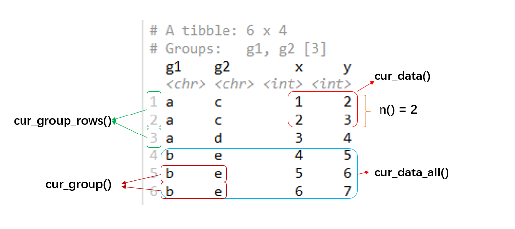
#> # … with 2 more rowsn()gives the current group size.gf %>% summarise(n = n()) #> `summarise()` has grouped output by 'g1'. You can override using the `.groups` argument. #> # A tibble: 3 x 3 #> # Groups: g1 [2] #> g1 g2 n #> <chr> <chr> <int> #> 1 a c 2 #> 2 a d 1 #> 3 b e 3cur_data()gives the current data for the current group (excluding grouping variables).gf %>% summarise(data = list(cur_data())) #> `summarise()` has grouped output by 'g1'. You can override using the `.groups` argument. #> # A tibble: 3 x 3 #> # Groups: g1 [2] #> g1 g2 data #> <chr> <chr> <list> #> 1 a c <tibble[,2] [2 × 2]> #> 2 a d <tibble[,2] [1 × 2]> #> 3 b e <tibble[,2] [3 × 2]>cur_data_all()gives the current data for the current group (including grouping variables).gf %>% summarise(data = list(cur_data_all())) #> `summarise()` has grouped output by 'g1'. You can override using the `.groups` argument. #> # A tibble: 3 x 3 #> # Groups: g1 [2] #> g1 g2 data #> <chr> <chr> <list> #> 1 a c <tibble[,4] [2 × 4]> #> 2 a d <tibble[,4] [1 × 4]> #> 3 b e <tibble[,4] [3 × 4]>cur_group()gives the group keys, a tibble with one row and one column for each grouping variable.gf %>% summarise(data = list(cur_group())) #> `summarise()` has grouped output by 'g1'. You can override using the `.groups` argument. #> # A tibble: 3 x 3 #> # Groups: g1 [2] #> g1 g2 data #> <chr> <chr> <list> #> 1 a c <tibble[,2] [1 × 2]> #> 2 a d <tibble[,2] [1 × 2]> #> 3 b e <tibble[,2] [1 × 2]>cur_group_id()gives a unique numeric identifier for the current group.gf %>% mutate(id = cur_group_id()) #> # A tibble: 6 x 5 #> # Groups: g1, g2 [3] #> g1 g2 x y id #> <chr> <chr> <int> <int> <int> #> 1 a c 1 2 1 #> 2 a c 2 3 1 #> 3 a d 3 4 2 #> 4 b e 4 5 3 #> # … with 2 more rowscur_group_rows()gives the row indices for the current group.gf %>% summarise(data = list(cur_group_rows())) #> `summarise()` has grouped output by 'g1'. You can override using the `.groups` argument. #> # A tibble: 3 x 3 #> # Groups: g1 [2] #> g1 g2 data #> <chr> <chr> <list> #> 1 a c <int [2]> #> 2 a d <int [1]> #> 3 b e <int [3]>
You can easily distinguish these functions in the following picture:
6.3 How group_by() works
group_by() create a new class of objects, grouped_df, who is treated differently with tbl_df, in most dplyr verbs.
df <- tibble(
  g1 = c('b', 'b', 'b', 'a', 'a', 'a'),
  g2 = c('c', 'c', 'd', 'e', 'e', 'e'),
  x = 1:6
)
gf <- df %>% group_by(g1, g2)

df %>% class()
#> [1] "tbl_df"     "tbl"        "data.frame"
gf %>% class()
#> [1] "grouped_df" "tbl_df"     "tbl"        "data.frame"
But group_by() never change the value of datasets (even the order of rows):
df
#> # A tibble: 6 x 3
#>   g1    g2        x
#>   <chr> <chr> <int>
#> 1 b     c         1
#> 2 b     c         2
#> 3 b     d         3
#> 4 a     e         4
#> # … with 2 more rows

gf
#> # A tibble: 6 x 3
#> # Groups:   g1, g2 [3]
#>   g1    g2        x
#>   <chr> <chr> <int>
#> 1 b     c         1
#> 2 b     c         2
#> 3 b     d         3
#> 4 a     e         4
#> # … with 2 more rows

df == gf
#>        g1   g2    x
#> [1,] TRUE TRUE TRUE
#> [2,] TRUE TRUE TRUE
#> [3,] TRUE TRUE TRUE
#> [4,] TRUE TRUE TRUE
#> [5,] TRUE TRUE TRUE
#> [6,] TRUE TRUE TRUE
Here we can easily notice that dplyr verbs have different behavior for df and gf:
df %>% mutate(sum = sum(x))
#> # A tibble: 6 x 4
#>   g1    g2        x   sum
#>   <chr> <chr> <int> <int>
#> 1 b     c         1    21
#> 2 b     c         2    21
#> 3 b     d         3    21
#> 4 a     e         4    21
#> # … with 2 more rows

gf %>% mutate(sum = sum(x))
#> # A tibble: 6 x 4
#> # Groups:   g1, g2 [3]
#>   g1    g2        x   sum
#>   <chr> <chr> <int> <int>
#> 1 b     c         1     3
#> 2 b     c         2     3
#> 3 b     d         3     3
#> 4 a     e         4    15
#> # … with 2 more rows
But in other places we should be cautious when we use a dataset output from a wrapped function, or write a function who receive an user-supplied data. For not knowing whether a grouped_df you get (or receive).
7 Row-wise operations
dplyr, and R in general, are particularly well suited to performing operations over columns, and performing operations over rows is much harder.
Let’s start from a little problem. We create a tibble df and want to calculate the sum of w x y z in each row:
df <- tibble(id = 1:6, w = 10:15, x = 20:25, y = 30:35, z = 40:45)

df %>% mutate(total = sum(c(w, x, y, z)))
#> # A tibble: 6 x 6
#>      id     w     x     y     z total
#>   <int> <int> <int> <int> <int> <int>
#> 1     1    10    20    30    40   660
#> 2     2    11    21    31    41   660
#> 3     3    12    22    32    42   660
#> 4     4    13    23    33    43   660
#> # … with 2 more rows
It doesn’t work out as expected, total calculate the sum of all value from w x y z (not in each row). This is because that sum() just return a single value calculated from the input:
sum(c(df$w, df$x, df$y, df$z))
#> [1] 660
then tibble treat the input as total = 660 and automatically recycle it.
The same problem will occur if you want to do row-wise aggregates with mean(), min(), max() and other functions who are not vectorised function. In order to solve this problem, you can use dplyr’s approach centred around the row-wise data frame created by rowwise().
7.1 rowwise()
Row-wise operations require a special type of grouping where each group consists of a single row. You create this with rowwise():
df %>% rowwise()
#> # A tibble: 6 x 5
#> # Rowwise:
#>      id     w     x     y     z
#>   <int> <int> <int> <int> <int>
#> 1     1    10    20    30    40
#> 2     2    11    21    31    41
#> 3     3    12    22    32    42
#> 4     4    13    23    33    43
#> # … with 2 more rows
Like group_by(), rowwise() doesn’t really do anything itself; it just changes how the other verbs work. For example, compare the results of mutate() in the following code:
df %>% mutate(total = sum(c(w, x, y, z)))
#> # A tibble: 6 x 6
#>      id     w     x     y     z total
#>   <int> <int> <int> <int> <int> <int>
#> 1     1    10    20    30    40   660
#> 2     2    11    21    31    41   660
#> 3     3    12    22    32    42   660
#> 4     4    13    23    33    43   660
#> # … with 2 more rows

df %>% rowwise() %>% mutate(total = sum(c(w, x, y, z)))
#> # A tibble: 6 x 6
#> # Rowwise:
#>      id     w     x     y     z total
#>   <int> <int> <int> <int> <int> <int>
#> 1     1    10    20    30    40   100
#> 2     2    11    21    31    41   104
#> 3     3    12    22    32    42   108
#> 4     4    13    23    33    43   112
#> # … with 2 more rows
If you use mutate() with a regular data frame, it computes the sum of w, x, y, and z across all rows. If you apply it to a row-wise data frame, it computes the sum for each row.
You can optionally supply “identifier” variables in your call to rowwise(). These variables are preserved when you call summarise(), so they behave somewhat similarly to the grouping variables passed to group_by():
df %>%
  rowwise() %>%
  summarise(total = sum(c(w, x, y, z)))
#> `summarise()` has ungrouped output. You can override using the `.groups` argument.
#> # A tibble: 6 x 1
#>   total
#>   <int>
#> 1   100
#> 2   104
#> 3   108
#> 4   112
#> # … with 2 more rows

df %>%
  rowwise(id) %>%
  summarise(total = sum(c(w, x, y, z)))
#> `summarise()` has grouped output by 'id'. You can override using the `.groups` argument.
#> # A tibble: 6 x 2
#> # Groups:   id [6]
#>      id total
#>   <int> <int>
#> 1     1   100
#> 2     2   104
#> 3     3   108
#> 4     4   112
#> # … with 2 more rows
rowwise() is just a special form of grouping, so if you want to remove it from a data frame, just call ungroup().
You can use c_across() which uses tidy selection syntax so you can to succinctly select many variables:
df %>%
  rowwise() %>%
  mutate(total = sum(c_across(w:z)))
#> # A tibble: 6 x 6
#> # Rowwise:
#>      id     w     x     y     z total
#>   <int> <int> <int> <int> <int> <int>
#> 1     1    10    20    30    40   100
#> 2     2    11    21    31    41   104
#> 3     3    12    22    32    42   108
#> 4     4    13    23    33    43   112
#> # … with 2 more rows
7.2 Other solution
The rowwise() approach will work for any summary function. But if you need greater speed, it’s worth looking for a built-in row-wise variant of your summary function. These are more efficient because they operate on the data frame as whole; they don’t split it into rows, compute the summary, and then join the results back together again.
df %>% mutate(total = rowSums(across(w:z)))
#> # A tibble: 6 x 6
#>      id     w     x     y     z total
#>   <int> <int> <int> <int> <int> <dbl>
#> 1     1    10    20    30    40   100
#> 2     2    11    21    31    41   104
#> 3     3    12    22    32    42   108
#> 4     4    13    23    33    43   112
#> # … with 2 more rows

df %>% mutate(mean = rowMeans(across(w:z)))
#> # A tibble: 6 x 6
#>      id     w     x     y     z  mean
#>   <int> <int> <int> <int> <int> <dbl>
#> 1     1    10    20    30    40    25
#> 2     2    11    21    31    41    26
#> 3     3    12    22    32    42    27
#> 4     4    13    23    33    43    28
#> # … with 2 more rowsNote: we don’t use rowwise() and use across() in rowMeans() and rowSums() here because across() returns a tibble and rowMeans() and rowSums() take a multi-row data frame as input.
Or you can use vectorised function, such as pmin(), pmax(). Similarly, they’ll be much faster than rowwise().
df %>% mutate(
  min = pmin(w, x, y, z),
  max = pmax(w, x, y, z)
)
#> # A tibble: 6 x 7
#>      id     w     x     y     z   min   max
#>   <int> <int> <int> <int> <int> <int> <int>
#> 1     1    10    20    30    40    10    40
#> 2     2    11    21    31    41    11    41
#> 3     3    12    22    32    42    12    42
#> 4     4    13    23    33    43    13    43
#> # … with 2 more rows
7.3 Difference between c_across(), across(), if_any() and if_all()
You can view the output structure of c_across(), across(), if_any() and if_all() by wrapping with list():
df %>% rowwise() %>% mutate(new = list(c_across(w:z)))
#> # A tibble: 6 x 6
#> # Rowwise:
#>      id     w     x     y     z new
#>   <int> <int> <int> <int> <int> <list>
#> 1     1    10    20    30    40 <int [4]>
#> 2     2    11    21    31    41 <int [4]>
#> 3     3    12    22    32    42 <int [4]>
#> 4     4    13    23    33    43 <int [4]>
#> # … with 2 more rows

df %>% rowwise() %>% mutate(new = list(across(w:z)))
#> # A tibble: 6 x 6
#> # Rowwise:
#>      id     w     x     y     z new
#>   <int> <int> <int> <int> <int> <list>
#> 1     1    10    20    30    40 <tibble[,4] [1 × 4]>
#> 2     2    11    21    31    41 <tibble[,4] [1 × 4]>
#> 3     3    12    22    32    42 <tibble[,4] [1 × 4]>
#> 4     4    13    23    33    43 <tibble[,4] [1 × 4]>
#> # … with 2 more rows

df %>% rowwise() %>% mutate(new = list(if_any(w:z, ~ .x > 25)))
#> # A tibble: 6 x 6
#> # Rowwise:
#>      id     w     x     y     z new
#>   <int> <int> <int> <int> <int> <list>
#> 1     1    10    20    30    40 <lgl [1]>
#> 2     2    11    21    31    41 <lgl [1]>
#> 3     3    12    22    32    42 <lgl [1]>
#> 4     4    13    23    33    43 <lgl [1]>
#> # … with 2 more rows


df %>% mutate(new = list(c_across(w:z)))
#> # A tibble: 6 x 6
#>      id     w     x     y     z new
#>   <int> <int> <int> <int> <int> <list>
#> 1     1    10    20    30    40 <int [24]>
#> 2     2    11    21    31    41 <int [24]>
#> 3     3    12    22    32    42 <int [24]>
#> 4     4    13    23    33    43 <int [24]>
#> # … with 2 more rows

df %>% mutate(new = list(across(w:z)))
#> # A tibble: 6 x 6
#>      id     w     x     y     z new
#>   <int> <int> <int> <int> <int> <list>
#> 1     1    10    20    30    40 <tibble[,4] [6 × 4]>
#> 2     2    11    21    31    41 <tibble[,4] [6 × 4]>
#> 3     3    12    22    32    42 <tibble[,4] [6 × 4]>
#> 4     4    13    23    33    43 <tibble[,4] [6 × 4]>
#> # … with 2 more rows

df %>% mutate(new = list(if_any(w:z, ~ .x > 25)))
#> # A tibble: 6 x 6
#>      id     w     x     y     z new
#>   <int> <int> <int> <int> <int> <list>
#> 1     1    10    20    30    40 <lgl [6]>
#> 2     2    11    21    31    41 <lgl [6]>
#> 3     3    12    22    32    42 <lgl [6]>
#> 4     4    13    23    33    43 <lgl [6]>
#> # … with 2 more rows
c_across() returns a vector, across() returns a tibble, if_any() and if_all() return a logical vector. We can also find that c_across() doesn’t work well without rowwise(). Use them cautiously depending on other function’s needed input.
8 Vector functions
8.1 Vectorised if: if_else() case_when()
if_else(condition, true, false, missing = NULL)
case_when(...)
x <- c(-5:5, NA)
if_else(x < 0, true = "negative", false = "positive", missing = "missing")
#>  [1] "negative" "negative" "negative" "negative" "negative" "positive"
#>  [7] "positive" "positive" "positive" "positive" "positive" "missing"

x <- 1:50
case_when(
  x %% 35 == 0 ~ "fizz buzz",
  x %% 5 == 0  ~ "fizz",
  x %% 7 == 0  ~ "buzz",
  TRUE         ~ as.character(x)
)
#>  [1] "1"         "2"         "3"         "4"         "fizz"      "6"
#>  [7] "buzz"      "8"         "9"         "fizz"      "11"        "12"
#> [13] "13"        "buzz"      "fizz"      "16"        "17"        "18"
#> [19] "19"        "fizz"      "buzz"      "22"        "23"        "24"
#> [25] "fizz"      "26"        "27"        "buzz"      "29"        "fizz"
#> [31] "31"        "32"        "33"        "34"        "fizz buzz" "36"
#> [37] "37"        "38"        "39"        "fizz"      "41"        "buzz"
#> [43] "43"        "44"        "fizz"      "46"        "47"        "48"
#> [49] "buzz"      "fizz"
If none of the cases match in case_when() (or do not clarify missing in if_else()), NA is used as return value:
x <- c(-1, 1, NA)

if_else(x < 0, 'negative', 'positive')
#> [1] "negative" "positive" NA

case_when(
  x < 0  ~ 'negative',
  x >= 0 ~ 'positive'
)
#> [1] "negative" "positive" NA
Use %>% with if_else() and case_when() (wrapped them with {}):
x <- c(-1, 1, NA)

x %>% {
  if_else(. < 0, "negative", "positive", "missing")
}
#> [1] "negative" "positive" "missing"

x %>% {
  case_when(
    . < 0  ~ "negative",
    . >= 0 ~ "positive",
    TRUE   ~ "missing"
  )
}
#> [1] "negative" "positive" "missing"
Note that if_else() and case_when() are both strict, if_else() checks that true and false are the same type, in case_when(), all RHSs must evaluate to the same type of vector. Inconsistent types will throw an error. This applies also to NA values used in RHS (or true false): NA is logical, use typed values like NA_real_, NA_complex_, NA_character_, NA_integer_ as appropriate.
x <- c(-1, 1)

case_when(
  x >= 0 ~ "positive",
  TRUE   ~ NA
)
#> Error: must be a character vector, not a logical vector.

case_when(
  x >= 0 ~ "positive",
  TRUE   ~ NA_character_
)
#> [1] NA         "positive"
if_else() and case_when() evaluates all expressions first, and then constructs its result by extracting the selected parts.
x <- -2:2 %>% as.double()

if_else(x >= 0, sqrt(x), x)
#> Warning in sqrt(x): NaNs produced
#> [1] -2.000000 -1.000000  0.000000  1.000000  1.414214

case_when(
  x >= 0 ~ sqrt(x),
  TRUE   ~ x
)
#> Warning in sqrt(x): NaNs produced
#> [1] -2.000000 -1.000000  0.000000  1.000000  1.414214
Sometimes it’s hard to generate multiple variables in complex condition statement via if_else() and case_when(), you can turn to use libr::datastep():
df <- tibble(x = 1:3, y = 4:6)

df %>% libr::datastep({
  if (x <= 2 & y == 4) {
    var1 <- 'a'
    var_temp <- 1
  } else {
    var1 <- 'b'
    var_temp <- 0
  }

  if (var_temp == 1 | x == 3) {
    var2 <- 'c'
  }

  rm(var_temp)
})
#> # A tibble: 3 x 4
#>       x     y var2  var1
#>   <int> <int> <chr> <chr>
#> 1     1     4 c     a
#> 2     2     5 <NA>  b
#> 3     3     6 c     b
8.2 Cumulativate functions: cumall() cumany() cummean()
Cumulative aggregates: cumsum(), cumprod(), cummin(), cummax() (from base R), and cumall(), cumany(), and cummean() (from dplyr).
cumsum(1:10)
#>  [1]  1  3  6 10 15 21 28 36 45 55

cumprod(1:5)
#> [1]   1   2   6  24 120

cummean(10:1)
#>  [1] 10.0  9.5  9.0  8.5  8.0  7.5  7.0  6.5  6.0  5.5

cummin(c(3, 2, 1, 2, 1, 0, 4, 3, 2))
#> [1] 3 2 1 1 1 0 0 0 0

cummax(c(3, 2, 1, 2, 1, 0, 4, 3, 2))
#> [1] 3 3 3 3 3 3 4 4 4

cumall(c(T, T, F, T, F))
#> [1] TRUE TRUE TRUE TRUE TRUE

cumany(c(F, F, T, F, T))
#> [1] TRUE TRUE TRUE TRUE TRUE
Cumulative logical functions cumall() and cumany() are particularly useful in conjunction with filter():
cumall(x): all cases until the firstFALSE.cumall(!x): all cases until the firstTRUE.cumany(x): all cases after the firstTRUE.cumany(!x): all cases after the firstFALSE.
df <- data.frame(
  date = as.Date("2020-01-01") + 0:6,
  balance = c(100, 50, 25, -25, -50, 30, 120)
)
df
#>         date balance
#> 1 2020-01-01     100
#> 2 2020-01-02      50
#> 3 2020-01-03      25
#> 4 2020-01-04     -25
#> 5 2020-01-05     -50
#> 6 2020-01-06      30
#> 7 2020-01-07     120

# all rows after first overdraft
df %>% filter(cumany(balance < 0))
#>         date balance
#> 1 2020-01-04     -25
#> 2 2020-01-05     -50
#> 3 2020-01-06      30
#> 4 2020-01-07     120

# all rows until first overdraft
df %>% filter(cumall(!(balance < 0)))
#>         date balance
#> 1 2020-01-01     100
#> 2 2020-01-02      50
#> 3 2020-01-03      25
8.3 Windowed rank functions: row_number() ntile() min_rank() dense_rank() percent_rank() cume_dist()
row_number(): equivalent torank(ties.method = "first")min_rank(): equivalent torank(ties.method = "min")dense_rank(): likemin_rank(), but with no gaps between rankspercent_rank(): a number between 0 and 1 computed by rescalingmin_rank()to[0, 1]cume_dist(): a cumulative distribution function. Proportion of all values less than or equal to the current rank.ntile(): a rough rank, which breaks the input vector intonbuckets. The size of the buckets may differ by up to one, larger buckets have lower rank.
x <- c(5, 1, 3, 2, 2)

row_number(x)
#> [1] 5 1 4 2 3

min_rank(x)
#> [1] 5 1 4 2 2

dense_rank(x)
#> [1] 4 1 3 2 2

percent_rank(x)
#> [1] 1.00 0.00 0.75 0.25 0.25

cume_dist(x)
#> [1] 1.0 0.2 0.8 0.6 0.6

ntile(x, 2)
#> [1] 2 1 2 1 1
ntile(1:8, 3)
#> [1] 1 1 1 2 2 2 3 3
All ranking functions rank from lowest to highest so that small input values get small ranks. Use desc() to rank from highest to lowest.
x <- c(5, 1, 3, 2, 2)

row_number(desc(x))
#> [1] 1 5 2 3 4

min_rank(desc(x))
#> [1] 1 5 2 3 3

dense_rank(desc(x))
#> [1] 1 4 2 3 3

percent_rank(desc(x))
#> [1] 0.00 1.00 0.25 0.50 0.50

cume_dist(desc(x))
#> [1] 0.2 1.0 0.4 0.8 0.8

ntile(desc(x), 2)
#> [1] 1 2 1 1 2
row_number() can be used with single table verbs without specifying x to denote the row number, and it would be affected by group_by():
starwars %>%
  select(name, species) %>%
  mutate(n = row_number())
#> # A tibble: 87 x 3
#>   name           species     n
#>   <chr>          <chr>   <int>
#> 1 Luke Skywalker Human       1
#> 2 C-3PO          Droid       2
#> 3 R2-D2          Droid       3
#> 4 Darth Vader    Human       4
#> # … with 83 more rows

starwars %>%
  select(name, species) %>%
  group_by(species) %>%
  mutate(n = row_number())
#> # A tibble: 87 x 3
#> # Groups:   species [38]
#>   name           species     n
#>   <chr>          <chr>   <int>
#> 1 Luke Skywalker Human       1
#> 2 C-3PO          Droid       1
#> 3 R2-D2          Droid       2
#> 4 Darth Vader    Human       2
#> # … with 83 more rows
8.4 Extract the first, last or nth value from a vector: nth() first() last()
first(x) last(x) nth(x, n)
x <- 1:10

first(x)
#> [1] 1
last(x)
#> [1] 10

nth(x, 1)
#> [1] 1
nth(x, 5)
#> [1] 5

nth(x, -2)
#> [1] 9

nth(x, 11)
#> [1] NA
8.5 Compute lagged or leading values: lag() lead()
lag(x, n = 1L, default = NA)
lead(x, n = 1L, default = NA)
lag(1:5)
#> [1] NA  1  2  3  4
lead(1:5)
#> [1]  2  3  4  5 NA

lag(1:5, n = 1)
#> [1] NA  1  2  3  4
lag(1:5, n = 2)
#> [1] NA NA  1  2  3

lead(1:5, n = 1)
#> [1]  2  3  4  5 NA
lead(1:5, n = 2)
#> [1]  3  4  5 NA NA

lag(1:5, default = 0)
#> [1] 0 1 2 3 4
lead(1:5, default = 6)
#> [1] 2 3 4 5 6
8.6 Find first non-missing element: coalesce()
y <- c(1, 2, NA, NA, 5, NA)
z <- c(NA, NA, 3, 4, 5, NA)
coalesce(y, z)
#> [1]  1  2  3  4  5 NA
You can use a single value to replace all missing values:
x <- sample(c(1:5, NA, NA, NA))
x
#> [1] NA NA  2 NA  5  1  3  4
coalesce(x, 0L)
#> [1] 0 0 2 0 5 1 3 4
8.7 Convert values to NA: na_if()
na_if(x, y)
x: Vector to modifyy: Value to replace withNA
na_if(1:5, 2)
#> [1]  1 NA  3  4  5

na_if(1:5, 5:1)
#> [1]  1  2 NA  4  5
8.8 Compare two numeric vectors: near()
near(x, y, tol = .Machine$double.eps^0.5)
sqrt(2) ^ 2 == 2
#> [1] FALSE

near(sqrt(2) ^ 2, 2)
#> [1] TRUE
8.9 Shortcut of left <= x & x <= right: between()
between(x, left, right)
between(1:12, 7, 9)
#>  [1] FALSE FALSE FALSE FALSE FALSE FALSE  TRUE  TRUE  TRUE FALSE FALSE FALSE
8.10 Efficiently count the number of unique values in a set of vector: n_distinct()
n_distinct(..., na.rm = FALSE)
x <- sample(1:10, 1e7, rep = TRUE)
n_distinct(x)
#> [1] 10

length(unique(x)) %>% system.time()
#>    user  system elapsed
#>   0.212   0.036   0.248

n_distinct(x) %>% system.time()
#>    user  system elapsed
#>   0.077   0.023   0.101