library(tidyverse)
packageVersion("tidyr")
#> [1] '1.1.3'

1 Separate and unite character vectors

1.1 Extract character column with regex groups: `extract()`

Given a regular expression with capturing groups, extract() turns each group into a new column. If the groups don’t match, or the input is NA, the output will be NA.

df <- tibble(folder = c('Screening', 'Cycle 1 Day 1', 'Cycle 2 Day 15'))
df
#> # A tibble: 3 x 1
#>   folder        
#>   <chr>         
#> 1 Screening     
#> 2 Cycle 1 Day 1 
#> 3 Cycle 2 Day 15

df %>% extract(
  col = folder,
  into = c('cycle', 'day'),
  regex = 'Cycle (\\d+) Day (\\d+)'
)
#> # A tibble: 3 x 2
#>   cycle day  
#>   <chr> <chr>
#> 1 <NA>  <NA> 
#> 2 1     1    
#> 3 2     15

df %>% extract(
  col = folder,
  into = c('cycle', 'day'),
  regex = 'Cycle (\\d+) Day (\\d+)',
  remove = F
)
#> # A tibble: 3 x 2
#>   cycle day  
#>   <chr> <chr>
#> 1 <NA>  <NA> 
#> 2 1     1    
#> 3 2     15

1.2 Separate character column with separator: `separate()`

Given either a regular expression or a vector of character positions, separate() turns a single character column into multiple columns.

regex separator

df <- tibble(x = c('a,b:c', 'd_e_f'))
df
#> # A tibble: 2 x 1
#>   x    
#>   <chr>
#> 1 a,b:c
#> 2 d_e_f

df %>% separate(
  col = x,
  into = c('x1', 'x2', 'x3'),
  sep = '[,:_]'
)
#> # A tibble: 2 x 3
#>   x1    x2    x3   
#>   <chr> <chr> <chr>
#> 1 a     b     c    
#> 2 d     e     f

df %>% separate(
  col = x,
  into = c('x1', 'x2', 'x3'),
  sep = '[,:_]',
  remove = F
)
#> # A tibble: 2 x 3
#>   x1    x2    x3   
#>   <chr> <chr> <chr>
#> 1 a     b     c    
#> 2 d     e     f

numeric vector is interpreted as character positions to split at.

df <- tibble(fruit = c('apple', 'orange', 'pear', 'banana'))
df
#> # A tibble: 4 x 1
#>   fruit 
#>   <chr> 
#> 1 apple 
#> 2 orange
#> 3 pear  
#> 4 banana

df %>% separate(
  col = fruit,
  into = c('var1', 'var2', 'var3'),
  sep = c(2, 5)
)
#> # A tibble: 4 x 3
#>   var1  var2  var3 
#>   <chr> <chr> <chr>
#> 1 ap    ple   ""   
#> 2 or    ang   "e"  
#> 3 pe    ar    ""   
#> 4 ba    nan   "a"

df %>% separate(
  col = fruit,
  into = c('var1', 'var2'),
  sep = -2
)
#> # A tibble: 4 x 2
#>   var1  var2 
#>   <chr> <chr>
#> 1 app   le   
#> 2 oran  ge   
#> 3 pe    ar   
#> 4 bana  na

You can use extra and fill when there are too many pieces (or not enough pieces):

extra: If sep is a character vector, this controls what happens when there are too many pieces. There are three valid options:

“warn” (the default): emit a warning and drop extra values.
“drop”: drop any extra values without a warning.

“merge”: only splits at most length(into) times

df <- tibble(fruits = c('apples, oranges, pears, bananas', 'pineapples, mangos, guavas'))
df
#> # A tibble: 2 x 1
#>   fruits                         
#>   <chr>                          
#> 1 apples, oranges, pears, bananas
#> 2 pineapples, mangos, guavas

df %>% separate(
  col = fruits,
  into = c('fruit1', 'fruit2'),
  sep = ', '
)
#> Warning: Expected 2 pieces. Additional pieces discarded in 2 rows [1, 2].
#> # A tibble: 2 x 2
#>   fruit1     fruit2 
#>   <chr>      <chr>  
#> 1 apples     oranges
#> 2 pineapples mangos

df %>% separate(
  col = fruits,
  into = c('fruit1', 'fruit2'),
  sep = ', ',
  extra = 'drop'
)
#> # A tibble: 2 x 2
#>   fruit1     fruit2 
#>   <chr>      <chr>  
#> 1 apples     oranges
#> 2 pineapples mangos

df %>% separate(
  col = fruits,
  into = c('fruit1', 'fruit2'),
  sep = ', ',
  extra = 'merge'
)
#> # A tibble: 2 x 2
#>   fruit1     fruit2                 
#>   <chr>      <chr>                  
#> 1 apples     oranges, pears, bananas
#> 2 pineapples mangos, guavas

fill: If sep is a character vector, this controls what happens when there are not enough pieces. There are three valid options:

“warn” (the default): emit a warning and fill from the right
“right”: fill with missing values on the right

“left”: fill with missing values on the left

df %>% separate(
  col = fruits,
  into = c('fruit1', 'fruit2', 'fruit3', 'fruit4', 'fruit5'),
  sep = ', '
)
#> Warning: Expected 5 pieces. Missing pieces filled with `NA` in 2 rows [1, 2].
#> # A tibble: 2 x 5
#>   fruit1     fruit2  fruit3 fruit4  fruit5
#>   <chr>      <chr>   <chr>  <chr>   <chr> 
#> 1 apples     oranges pears  bananas <NA>  
#> 2 pineapples mangos  guavas <NA>    <NA>

df %>% separate(
  col = fruits,
  into = c('fruit1', 'fruit2', 'fruit3', 'fruit4', 'fruit5'),
  sep = ', ',
  fill = 'right'
)
#> # A tibble: 2 x 5
#>   fruit1     fruit2  fruit3 fruit4  fruit5
#>   <chr>      <chr>   <chr>  <chr>   <chr> 
#> 1 apples     oranges pears  bananas <NA>  
#> 2 pineapples mangos  guavas <NA>    <NA>

df %>% separate(
  col = fruits,
  into = c('fruit1', 'fruit2', 'fruit3', 'fruit4', 'fruit5'),
  sep = ', ',
  fill = 'left'
)
#> # A tibble: 2 x 5
#>   fruit1 fruit2 fruit3     fruit4 fruit5 
#>   <chr>  <chr>  <chr>      <chr>  <chr>  
#> 1 <NA>   apples oranges    pears  bananas
#> 2 <NA>   <NA>   pineapples mangos guavas

1.3 Separate character column into multiple rows: `separate_rows()`

df <- tibble(
  id = 1:2,
  fruits = c(
    "apples and oranges and pears and bananas",
    "pineapples and mangos and guavas"
  )
)
df
#> # A tibble: 2 x 2
#>      id fruits                                  
#>   <int> <chr>                                   
#> 1     1 apples and oranges and pears and bananas
#> 2     2 pineapples and mangos and guavas

df %>% separate_rows(fruits, sep = ' and ')
#> # A tibble: 7 x 2
#>      id fruits    
#>   <int> <chr>     
#> 1     1 apples    
#> 2     1 oranges   
#> 3     1 pears     
#> 4     1 bananas   
#> 5     2 pineapples
#> 6     2 mangos    
#> 7     2 guavas

1.4 Unite multiple columns into one: `unite()`

df <- tibble(x = c('a', 'b'), y = c('c', 'd'), z = c('e', 'f'))
df
#> # A tibble: 2 x 3
#>   x     y     z    
#>   <chr> <chr> <chr>
#> 1 a     c     e    
#> 2 b     d     f

df %>% unite(xy, c(x, y), sep = '_')
#> # A tibble: 2 x 2
#>   xy    z    
#>   <chr> <chr>
#> 1 a_c   e    
#> 2 b_d   f

df %>% unite(xyz, x:z, sep = '.')
#> # A tibble: 2 x 1
#>   xyz  
#>   <chr>
#> 1 a.c.e
#> 2 b.d.f

df %>% unite(xyz, x:z, sep = '.', remove = F)
#> # A tibble: 2 x 1
#>   xyz  
#>   <chr>
#> 1 a.c.e
#> 2 b.d.f

You can use na.rm to remove missing values:

df <- tibble(x = c('a', 'b', 'c'), y = c('d', 'e', NA))
df
#> # A tibble: 3 x 2
#>   x     y    
#>   <chr> <chr>
#> 1 a     d    
#> 2 b     e    
#> 3 c     <NA>

df %>% unite(xy, c(x, y), sep = '_')
#> # A tibble: 3 x 1
#>   xy   
#>   <chr>
#> 1 a_d  
#> 2 b_e  
#> 3 c_NA

df %>% unite(xy, c(x, y), sep = '_', na.rm = T)
#> # A tibble: 3 x 1
#>   xy   
#>   <chr>
#> 1 a_d  
#> 2 b_e  
#> 3 c

2 Handle missing values

2.1 Drop rows containing missing values: `drop_na()`

df <- tibble(x = c(1, 2, NA), y = c("a", NA, "b"))
df
#> # A tibble: 3 x 2
#>       x y    
#>   <dbl> <chr>
#> 1     1 a    
#> 2     2 <NA> 
#> 3    NA b

df %>% drop_na()
#> # A tibble: 1 x 2
#>       x y    
#>   <dbl> <chr>
#> 1     1 a

df %>% drop_na(x)
#> # A tibble: 2 x 2
#>       x y    
#>   <dbl> <chr>
#> 1     1 a    
#> 2     2 <NA>

2.2 Replace NAs with specified values: `replace_na()`

Replace NAs for vector

x <- c('a', 'b', NA)
replace_na(x, 'missing')
#> [1] "a"       "b"       "missing"

Replace NAs for dataframe

df <- tibble(x = c(1, 2, NA), y = c("a", NA, "b"))
df
#> # A tibble: 3 x 2
#>       x y    
#>   <dbl> <chr>
#> 1     1 a    
#> 2     2 <NA> 
#> 3    NA b

df %>% replace_na(list(x = 0, y = "unknown"))
#> # A tibble: 3 x 2
#>       x y      
#>   <dbl> <chr>  
#> 1     1 a      
#> 2     2 unknown
#> 3     0 b

2.3 Fill in missing values with previous or next value: `fill()`

You can fill missing values in selected columns using the next or previous entry. The direction can be chose as “down” (the default), “up”, “downup” (i.e. first down and then up) or “updown” (first up and then down).

df <- tribble(
  ~quarter, ~year, ~sales,
  "Q1",      NA,    66013,
  "Q2",      NA,    69182,
  "Q3",    2000,    53175,
  "Q4",      NA,    21001,
  "Q1",    2001,    46036,
  "Q2",      NA,    58842,
  "Q3",      NA,    44568,
  "Q4",      NA,    50197,
)

df %>% fill(year)
#> # A tibble: 8 x 3
#>   quarter  year sales
#>   <chr>   <dbl> <dbl>
#> 1 Q1         NA 66013
#> 2 Q2         NA 69182
#> 3 Q3       2000 53175
#> 4 Q4       2000 21001
#> 5 Q1       2001 46036
#> 6 Q2       2001 58842
#> 7 Q3       2001 44568
#> 8 Q4       2001 50197

df %>% fill(year, .direction = 'up')
#> # A tibble: 8 x 3
#>   quarter  year sales
#>   <chr>   <dbl> <dbl>
#> 1 Q1       2000 66013
#> 2 Q2       2000 69182
#> 3 Q3       2000 53175
#> 4 Q4       2001 21001
#> 5 Q1       2001 46036
#> 6 Q2         NA 58842
#> 7 Q3         NA 44568
#> 8 Q4         NA 50197

df %>% fill(year, .direction = 'downup')
#> # A tibble: 8 x 3
#>   quarter  year sales
#>   <chr>   <dbl> <dbl>
#> 1 Q1       2000 66013
#> 2 Q2       2000 69182
#> 3 Q3       2000 53175
#> 4 Q4       2000 21001
#> 5 Q1       2001 46036
#> 6 Q2       2001 58842
#> 7 Q3       2001 44568
#> 8 Q4       2001 50197

You can use fill() to “retain” value from previous observations. For example, you can get the dosage from latest cycle (dosage who is not 0 or NA):

df <- tibble(cycle = 1:7, dose = c(1, 0, NA, 2, 3, NA, 4))
df
#> # A tibble: 7 x 2
#>   cycle  dose
#>   <int> <dbl>
#> 1     1     1
#> 2     2     0
#> 3     3    NA
#> 4     4     2
#> 5     5     3
#> 6     6    NA
#> 7     7     4

df %>% 
  mutate(
    last_dose = if_else(dose %in% c(0, NA), NA_real_, dose),
    last_dose = lag(last_dose)
  ) %>% 
  fill(last_dose)
#> # A tibble: 7 x 3
#>   cycle  dose last_dose
#>   <int> <dbl>     <dbl>
#> 1     1     1        NA
#> 2     2     0         1
#> 3     3    NA         1
#> 4     4     2         1
#> 5     5     3         2
#> 6     6    NA         3
#> 7     7     4         3

3 Reshape data

3.1 Pivot data from wide to long: `pivot_longer()`

pivot_longer() “Lengthen” data by collapsing several columns into two. You can select columns by cols with <tidy-select>, column names move to a new names_to column and values to a new values_to column.

pivot_longer(
  data,
  cols,
  names_to = "name",
  names_prefix = NULL,
  names_sep = NULL,
  names_pattern = NULL,
  values_to = "value",
  values_drop_na = FALSE
)

Simplest case

table4a
#> # A tibble: 3 x 3
#>   country     `1999` `2000`
#> * <chr>        <int>  <int>
#> 1 Afghanistan    745   2666
#> 2 Brazil       37737  80488
#> 3 China       212258 213766

table4a %>% pivot_longer(c(`1999`, `2000`), names_to = 'year', values_to = 'cases')
#> # A tibble: 6 x 3
#>   country     year   cases
#>   <chr>       <chr>  <int>
#> 1 Afghanistan 1999     745
#> 2 Afghanistan 2000    2666
#> 3 Brazil      1999   37737
#> 4 Brazil      2000   80488
#> 5 China       1999  212258
#> 6 China       2000  213766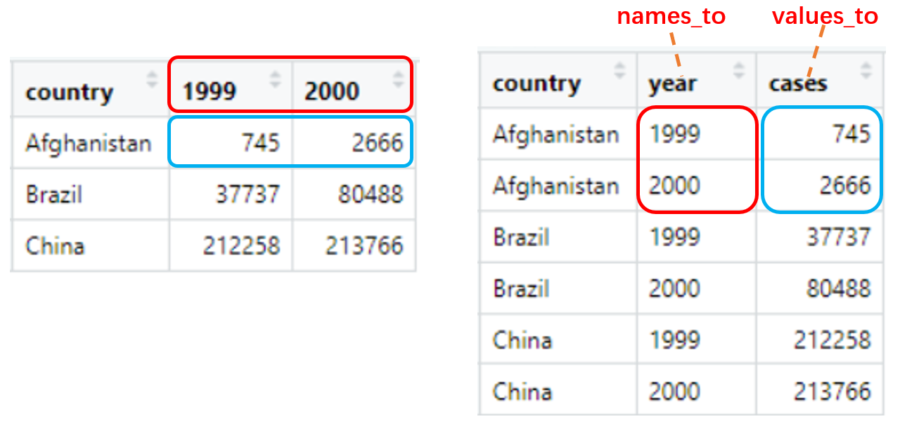

Drop rows that correspond to missing values

You can drop rows that contain only NA in the values_to column:

df <- tribble(
  ~id, ~choice1, ~choice2, ~choice3,
  1, "A", "B", "C",
  2, "C", "B",  NA,
  3, "D",  NA,  NA,
  4, "B", "D",  NA
)

df %>% pivot_longer(!id)
#> # A tibble: 12 x 3
#>       id name    value
#>    <dbl> <chr>   <chr>
#>  1     1 choice1 A    
#>  2     1 choice2 B    
#>  3     1 choice3 C    
#>  4     2 choice1 C    
#>  5     2 choice2 B    
#>  6     2 choice3 <NA> 
#>  7     3 choice1 D    
#>  8     3 choice2 <NA> 
#>  9     3 choice3 <NA> 
#> 10     4 choice1 B    
#> # … with 2 more rows

df %>% pivot_longer(!id, values_drop_na = T)
#> # A tibble: 8 x 3
#>      id name    value
#>   <dbl> <chr>   <chr>
#> 1     1 choice1 A    
#> 2     1 choice2 B    
#> 3     1 choice3 C    
#> 4     2 choice1 C    
#> 5     2 choice2 B    
#> 6     3 choice1 D    
#> 7     4 choice1 B    
#> 8     4 choice2 D

strip common prefix

You can use names_prefix to strip common prefix:

billboard
#> # A tibble: 317 x 79
#>    artist   track   date.entered   wk1   wk2   wk3   wk4   wk5   wk6   wk7   wk8
#>    <chr>    <chr>   <date>       <dbl> <dbl> <dbl> <dbl> <dbl> <dbl> <dbl> <dbl>
#>  1 2 Pac    Baby D… 2000-02-26      87    82    72    77    87    94    99    NA
#>  2 2Ge+her  The Ha… 2000-09-02      91    87    92    NA    NA    NA    NA    NA
#>  3 3 Doors… Krypto… 2000-04-08      81    70    68    67    66    57    54    53
#>  4 3 Doors… Loser   2000-10-21      76    76    72    69    67    65    55    59
#>  5 504 Boyz Wobble… 2000-04-15      57    34    25    17    17    31    36    49
#>  6 98^0     Give M… 2000-08-19      51    39    34    26    26    19     2     2
#>  7 A*Teens  Dancin… 2000-07-08      97    97    96    95   100    NA    NA    NA
#>  8 Aaliyah  I Don'… 2000-01-29      84    62    51    41    38    35    35    38
#>  9 Aaliyah  Try Ag… 2000-03-18      59    53    38    28    21    18    16    14
#> 10 Adams, … Open M… 2000-08-26      76    76    74    69    68    67    61    58
#> # … with 307 more rows, and 68 more variables: wk9 <dbl>, wk10 <dbl>,
#> #   wk11 <dbl>, wk12 <dbl>, wk13 <dbl>, wk14 <dbl>, wk15 <dbl>, wk16 <dbl>,
#> #   wk17 <dbl>, wk18 <dbl>, wk19 <dbl>, wk20 <dbl>, wk21 <dbl>, wk22 <dbl>,
#> #   wk23 <dbl>, wk24 <dbl>, wk25 <dbl>, wk26 <dbl>, wk27 <dbl>, wk28 <dbl>,
#> #   wk29 <dbl>, wk30 <dbl>, wk31 <dbl>, wk32 <dbl>, wk33 <dbl>, wk34 <dbl>,
#> #   wk35 <dbl>, wk36 <dbl>, wk37 <dbl>, wk38 <dbl>, wk39 <dbl>, wk40 <dbl>,
#> #   wk41 <dbl>, wk42 <dbl>, wk43 <dbl>, wk44 <dbl>, wk45 <dbl>, wk46 <dbl>,
#> #   wk47 <dbl>, wk48 <dbl>, wk49 <dbl>, wk50 <dbl>, wk51 <dbl>, wk52 <dbl>,
#> #   wk53 <dbl>, wk54 <dbl>, wk55 <dbl>, wk56 <dbl>, wk57 <dbl>, wk58 <dbl>,
#> #   wk59 <dbl>, wk60 <dbl>, wk61 <dbl>, wk62 <dbl>, wk63 <dbl>, wk64 <dbl>,
#> #   wk65 <dbl>, wk66 <lgl>, wk67 <lgl>, wk68 <lgl>, wk69 <lgl>, wk70 <lgl>,
#> #   wk71 <lgl>, wk72 <lgl>, wk73 <lgl>, wk74 <lgl>, wk75 <lgl>, wk76 <lgl>

billboard %>% 
  pivot_longer(
    cols = starts_with("wk"), 
    names_to = "week",
    names_prefix = 'wk', 
    values_to = "rank",
    values_drop_na = T
  )
#> # A tibble: 5,307 x 5
#>    artist  track                   date.entered week   rank
#>    <chr>   <chr>                   <date>       <chr> <dbl>
#>  1 2 Pac   Baby Don't Cry (Keep... 2000-02-26   1        87
#>  2 2 Pac   Baby Don't Cry (Keep... 2000-02-26   2        82
#>  3 2 Pac   Baby Don't Cry (Keep... 2000-02-26   3        72
#>  4 2 Pac   Baby Don't Cry (Keep... 2000-02-26   4        77
#>  5 2 Pac   Baby Don't Cry (Keep... 2000-02-26   5        87
#>  6 2 Pac   Baby Don't Cry (Keep... 2000-02-26   6        94
#>  7 2 Pac   Baby Don't Cry (Keep... 2000-02-26   7        99
#>  8 2Ge+her The Hardest Part Of ... 2000-09-02   1        91
#>  9 2Ge+her The Hardest Part Of ... 2000-09-02   2        87
#> 10 2Ge+her The Hardest Part Of ... 2000-09-02   3        92
#> # … with 5,297 more rows

Multiple variables stored in column names

You can extract multiple names_to columns via names_sep or names_pattern, for example, “sex” and “level” stored as column names and separated by _:

df <- tribble(
  ~subject,  ~f_1,  ~f_2, ~m_1, ~m_2,
         1,    11,    21,   31,   41,
         2,    12,    22,   32,   42,
         3,    13,    23,   33,   43,
)

df %>% 
  pivot_longer(
    cols = !subject,
    names_to = c('sex', 'level'),
    names_sep = '_'
  )
#> # A tibble: 12 x 4
#>    subject sex   level value
#>      <dbl> <chr> <chr> <dbl>
#>  1       1 f     1        11
#>  2       1 f     2        21
#>  3       1 m     1        31
#>  4       1 m     2        41
#>  5       2 f     1        12
#>  6       2 f     2        22
#>  7       2 m     1        32
#>  8       2 m     2        42
#>  9       3 f     1        13
#> 10       3 f     2        23
#> # … with 2 more rows

df %>% 
  pivot_longer(
    cols = !subject,
    names_to = c('sex', 'level'),
    names_pattern = '(.)_(.)'
  )
#> # A tibble: 12 x 4
#>    subject sex   level value
#>      <dbl> <chr> <chr> <dbl>
#>  1       1 f     1        11
#>  2       1 f     2        21
#>  3       1 m     1        31
#>  4       1 m     2        41
#>  5       2 f     1        12
#>  6       2 f     2        22
#>  7       2 m     1        32
#>  8       2 m     2        42
#>  9       3 f     1        13
#> 10       3 f     2        23
#> # … with 2 more rows

names_sep and names_pattern work same as separate() and extract(), you can also use separate() or extract() after pivot_longer():

df %>% 
  pivot_longer(cols = !subject) %>% 
  separate(col = 'name', into = c('sex', 'level'), sep = '_')
#> # A tibble: 12 x 4
#>    subject sex   level value
#>      <dbl> <chr> <chr> <dbl>
#>  1       1 f     1        11
#>  2       1 f     2        21
#>  3       1 m     1        31
#>  4       1 m     2        41
#>  5       2 f     1        12
#>  6       2 f     2        22
#>  7       2 m     1        32
#>  8       2 m     2        42
#>  9       3 f     1        13
#> 10       3 f     2        23
#> # … with 2 more rows

df %>% 
  pivot_longer(cols = !subject) %>% 
  extract(col = 'name', into = c('sex', 'level'), regex = '(.)_(.)')
#> # A tibble: 12 x 4
#>    subject sex   level value
#>      <dbl> <chr> <chr> <dbl>
#>  1       1 f     1        11
#>  2       1 f     2        21
#>  3       1 m     1        31
#>  4       1 m     2        41
#>  5       2 f     1        12
#>  6       2 f     2        22
#>  7       2 m     1        32
#>  8       2 m     2        42
#>  9       3 f     1        13
#> 10       3 f     2        23
#> # … with 2 more rows

Multiple group of columns to pivot

family <- tribble(
  ~family,  ~dob_child1,  ~dob_child2, ~gender_child1, ~gender_child2,
       1L, "1998-11-26", "2000-01-29",             1L,             2L,
       2L, "1996-06-22",           NA,             2L,             NA,
       3L, "2002-07-11", "2004-04-05",             2L,             2L,
       4L, "2004-10-10", "2009-08-27",             1L,             1L,
       5L, "2000-12-05", "2005-02-28",             2L,             1L,
)

We have two pieces of information (or values) for each child: their gender and their dob, these need to go into separate columns in the result. Here we use names_sep to split up each variable name, use a special name .value in names_to to extract the name of the “value” columns, and ignore the argument values_to.

family %>% 
  pivot_longer(
    !family, 
    names_to = c(".value", "child"), 
    names_sep = "_", 
    values_drop_na = TRUE
  )
#> # A tibble: 9 x 4
#>   family child  dob        gender
#>    <int> <chr>  <chr>       <int>
#> 1      1 child1 1998-11-26      1
#> 2      1 child2 2000-01-29      2
#> 3      2 child1 1996-06-22      2
#> 4      3 child1 2002-07-11      2
#> 5      3 child2 2004-04-05      2
#> 6      4 child1 2004-10-10      1
#> 7      4 child2 2009-08-27      1
#> 8      5 child1 2000-12-05      2
#> 9      5 child2 2005-02-28      1

3.2 Pivot data from long to wide: `pivot_wider()`

pivot_wider() “Widen” data by expanding two columns into several. names_from provides the new column names and values_from provides the values.

pivot_wider(
  data,
  id_cols = NULL,
  names_from = name,
  names_prefix = "",
  names_sep = "_",
  names_glue = NULL,
  values_from = value,
  values_fill = NULL
)

3.2.1 Simplest case

table2
#> # A tibble: 12 x 4
#>    country      year type            count
#>    <chr>       <int> <chr>           <int>
#>  1 Afghanistan  1999 cases             745
#>  2 Afghanistan  1999 population   19987071
#>  3 Afghanistan  2000 cases            2666
#>  4 Afghanistan  2000 population   20595360
#>  5 Brazil       1999 cases           37737
#>  6 Brazil       1999 population  172006362
#>  7 Brazil       2000 cases           80488
#>  8 Brazil       2000 population  174504898
#>  9 China        1999 cases          212258
#> 10 China        1999 population 1272915272
#> # … with 2 more rows

table2 %>% pivot_wider(names_from = type, values_from = count)
#> # A tibble: 6 x 4
#>   country      year  cases population
#>   <chr>       <int>  <int>      <int>
#> 1 Afghanistan  1999    745   19987071
#> 2 Afghanistan  2000   2666   20595360
#> 3 Brazil       1999  37737  172006362
#> 4 Brazil       2000  80488  174504898
#> 5 China        1999 212258 1272915272
#> 6 China        2000 213766 1280428583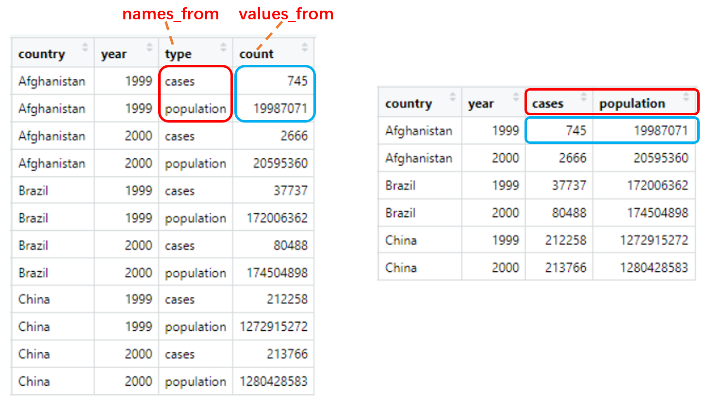

3.2.2 Fill in missing values

You can fill in missing values with values_fill:

fish_encounters
#> # A tibble: 114 x 3
#>    fish  station  seen
#>    <fct> <fct>   <int>
#>  1 4842  Release     1
#>  2 4842  I80_1       1
#>  3 4842  Lisbon      1
#>  4 4842  Rstr        1
#>  5 4842  Base_TD     1
#>  6 4842  BCE         1
#>  7 4842  BCW         1
#>  8 4842  BCE2        1
#>  9 4842  BCW2        1
#> 10 4842  MAE         1
#> # … with 104 more rows

fish_encounters %>% pivot_wider(names_from = station, values_from = seen)
#> # A tibble: 19 x 12
#>    fish  Release I80_1 Lisbon  Rstr Base_TD   BCE   BCW  BCE2  BCW2   MAE   MAW
#>    <fct>   <int> <int>  <int> <int>   <int> <int> <int> <int> <int> <int> <int>
#>  1 4842        1     1      1     1       1     1     1     1     1     1     1
#>  2 4843        1     1      1     1       1     1     1     1     1     1     1
#>  3 4844        1     1      1     1       1     1     1     1     1     1     1
#>  4 4845        1     1      1     1       1    NA    NA    NA    NA    NA    NA
#>  5 4847        1     1      1    NA      NA    NA    NA    NA    NA    NA    NA
#>  6 4848        1     1      1     1      NA    NA    NA    NA    NA    NA    NA
#>  7 4849        1     1     NA    NA      NA    NA    NA    NA    NA    NA    NA
#>  8 4850        1     1     NA     1       1     1     1    NA    NA    NA    NA
#>  9 4851        1     1     NA    NA      NA    NA    NA    NA    NA    NA    NA
#> 10 4854        1     1     NA    NA      NA    NA    NA    NA    NA    NA    NA
#> # … with 9 more rows

fish_encounters %>% pivot_wider(names_from = station, values_from = seen, values_fill = 0)
#> # A tibble: 19 x 12
#>    fish  Release I80_1 Lisbon  Rstr Base_TD   BCE   BCW  BCE2  BCW2   MAE   MAW
#>    <fct>   <int> <int>  <int> <int>   <int> <int> <int> <int> <int> <int> <int>
#>  1 4842        1     1      1     1       1     1     1     1     1     1     1
#>  2 4843        1     1      1     1       1     1     1     1     1     1     1
#>  3 4844        1     1      1     1       1     1     1     1     1     1     1
#>  4 4845        1     1      1     1       1     0     0     0     0     0     0
#>  5 4847        1     1      1     0       0     0     0     0     0     0     0
#>  6 4848        1     1      1     1       0     0     0     0     0     0     0
#>  7 4849        1     1      0     0       0     0     0     0     0     0     0
#>  8 4850        1     1      0     1       1     1     1     0     0     0     0
#>  9 4851        1     1      0     0       0     0     0     0     0     0     0
#> 10 4854        1     1      0     0       0     0     0     0     0     0     0
#> # … with 9 more rows

3.2.3 Generate column name from multiple variables

When names_from or values_from contains multiple variables, names_sep or names_glue can be used to generate the new column names.

use names_sep or names_glue to combine multiple names_from:

production <- expand_grid(
    product = c("A", "B"), 
    country = c("AI", "EI"), 
    year = 2000:2014
  ) %>%
  filter((product == "A" & country == "AI") | product == "B") %>% 
  mutate(production = rnorm(n()))

production
#> # A tibble: 45 x 4
#>    product country  year production
#>    <chr>   <chr>   <int>      <dbl>
#>  1 A       AI       2000      0.896
#>  2 A       AI       2001      0.732
#>  3 A       AI       2002     -0.308
#>  4 A       AI       2003     -0.951
#>  5 A       AI       2004     -0.356
#>  6 A       AI       2005      1.32 
#>  7 A       AI       2006     -0.125
#>  8 A       AI       2007      0.515
#>  9 A       AI       2008      0.667
#> 10 A       AI       2009     -0.464
#> # … with 35 more rows

production %>% pivot_wider(
  names_from = c(product, country), 
  values_from = production,
  names_sep = "."
)
#> # A tibble: 15 x 4
#>     year   A.AI      B.AI    B.EI
#>    <int>  <dbl>     <dbl>   <dbl>
#>  1  2000  0.896 -0.0120   -0.366 
#>  2  2001  0.732 -0.993    -0.639 
#>  3  2002 -0.308 -0.306     0.952 
#>  4  2003 -0.951  0.159    -0.484 
#>  5  2004 -0.356 -0.000914 -0.680 
#>  6  2005  1.32  -0.672     0.200 
#>  7  2006 -0.125  2.65     -0.0429
#>  8  2007  0.515  2.00      0.509 
#>  9  2008  0.667  1.41     -1.16  
#> 10  2009 -0.464  0.604     0.846 
#> # … with 5 more rows

production %>% pivot_wider(
  names_from = c(product, country), 
  values_from = production,
  names_glue = "{country}_{product}"
)
#> # A tibble: 15 x 4
#>     year   AI_A      AI_B    EI_B
#>    <int>  <dbl>     <dbl>   <dbl>
#>  1  2000  0.896 -0.0120   -0.366 
#>  2  2001  0.732 -0.993    -0.639 
#>  3  2002 -0.308 -0.306     0.952 
#>  4  2003 -0.951  0.159    -0.484 
#>  5  2004 -0.356 -0.000914 -0.680 
#>  6  2005  1.32  -0.672     0.200 
#>  7  2006 -0.125  2.65     -0.0429
#>  8  2007  0.515  2.00      0.509 
#>  9  2008  0.667  1.41     -1.16  
#> 10  2009 -0.464  0.604     0.846 
#> # … with 5 more rows

use multiple values_from to pivot groups of columns:

us_rent_income
#> # A tibble: 104 x 5
#>    GEOID NAME       variable estimate   moe
#>    <chr> <chr>      <chr>       <dbl> <dbl>
#>  1 01    Alabama    income      24476   136
#>  2 01    Alabama    rent          747     3
#>  3 02    Alaska     income      32940   508
#>  4 02    Alaska     rent         1200    13
#>  5 04    Arizona    income      27517   148
#>  6 04    Arizona    rent          972     4
#>  7 05    Arkansas   income      23789   165
#>  8 05    Arkansas   rent          709     5
#>  9 06    California income      29454   109
#> 10 06    California rent         1358     3
#> # … with 94 more rows

us_rent_income %>%
  pivot_wider(
    names_from = variable,
    names_glue = "{variable}_{.value}",
    values_from = c(estimate, moe)
  )
#> # A tibble: 52 x 6
#>    GEOID NAME                 income_estimate rent_estimate income_moe rent_moe
#>    <chr> <chr>                          <dbl>         <dbl>      <dbl>    <dbl>
#>  1 01    Alabama                        24476           747        136        3
#>  2 02    Alaska                         32940          1200        508       13
#>  3 04    Arizona                        27517           972        148        4
#>  4 05    Arkansas                       23789           709        165        5
#>  5 06    California                     29454          1358        109        3
#>  6 08    Colorado                       32401          1125        109        5
#>  7 09    Connecticut                    35326          1123        195        5
#>  8 10    Delaware                       31560          1076        247       10
#>  9 11    District of Columbia           43198          1424        681       17
#> 10 12    Florida                        25952          1077         70        3
#> # … with 42 more rows

3.3 longer then wider

You can combine pivot_longer() and pivot_wider() for more complex problems:

df <- tribble(
  ~ group, ~ level1, ~ level2,
      'a',        3,        4,
      'b',       50,      100,
      'c',      200,     1000,
)

df %>% pivot_longer(starts_with('level'), names_to = 'level', values_to = 'value')
#> # A tibble: 6 x 3
#>   group level  value
#>   <chr> <chr>  <dbl>
#> 1 a     level1     3
#> 2 a     level2     4
#> 3 b     level1    50
#> 4 b     level2   100
#> 5 c     level1   200
#> 6 c     level2  1000

df %>% 
  pivot_longer(starts_with('level'), names_to = 'level', values_to = 'value') %>% 
  pivot_wider(names_from = 'group', values_from = 'value')
#> # A tibble: 2 x 4
#>   level      a     b     c
#>   <chr>  <dbl> <dbl> <dbl>
#> 1 level1     3    50   200
#> 2 level2     4   100  1000

3.4 Using pivotting specification

To gain more control over pivotting, you can create a “spec” data frame that describes exactly how data stored in the column names becomes variables (and vice versa).

You can refer to Pivoting | Manual specs

4 Generate “complete” data

4.1 Create tibble from all combinations of inputs: `expand_grid()`

expand_grid(x = 1:2, y = c('a', 'b', 'c'))
#> # A tibble: 6 x 2
#>       x y    
#>   <int> <chr>
#> 1     1 a    
#> 2     1 b    
#> 3     1 c    
#> 4     2 a    
#> 5     2 b    
#> 6     2 c

expand_grid(var1 = c(1, 2, 1), var2 = c('a', 'b'))
#> # A tibble: 6 x 2
#>    var1 var2 
#>   <dbl> <chr>
#> 1     1 a    
#> 2     1 b    
#> 3     2 a    
#> 4     2 b    
#> 5     1 a    
#> 6     1 b

4.2 Expand data frame to include all possible combinations of values: `expand()`

expand() generates all combination of variables found in a dataset, and drop other columns:

fruits <- tibble(
  type   = c("apple", "orange", "apple", "orange", "orange", "orange"),
  year   = c(2010, 2010, 2012, 2010, 2010, 2012),
  size  =  c("XS", "S",  "M", "S", "S", "M")
)

fruits %>% expand(type, year)
#> # A tibble: 4 x 2
#>   type    year
#>   <chr>  <dbl>
#> 1 apple   2010
#> 2 apple   2012
#> 3 orange  2010
#> 4 orange  2012

fruits %>% expand(type, year, size)
#> # A tibble: 12 x 3
#>    type    year size 
#>    <chr>  <dbl> <chr>
#>  1 apple   2010 M    
#>  2 apple   2010 S    
#>  3 apple   2010 XS   
#>  4 apple   2012 M    
#>  5 apple   2012 S    
#>  6 apple   2012 XS   
#>  7 orange  2010 M    
#>  8 orange  2010 S    
#>  9 orange  2010 XS   
#> 10 orange  2012 M    
#> # … with 2 more rows

It’s same as using expand_grid() and unique() out of the dataset:

expand_grid(type = unique(fruits$type), year = unique(fruits$year))
#> # A tibble: 4 x 2
#>   type    year
#>   <chr>  <dbl>
#> 1 apple   2010
#> 2 apple   2012
#> 3 orange  2010
#> 4 orange  2012

expand_grid(type = unique(fruits$type), year = unique(fruits$year), size = unique(fruits$size))
#> # A tibble: 12 x 3
#>    type    year size 
#>    <chr>  <dbl> <chr>
#>  1 apple   2010 XS   
#>  2 apple   2010 S    
#>  3 apple   2010 M    
#>  4 apple   2012 XS   
#>  5 apple   2012 S    
#>  6 apple   2012 M    
#>  7 orange  2010 XS   
#>  8 orange  2010 S    
#>  9 orange  2010 M    
#> 10 orange  2012 XS   
#> # … with 2 more rows

You can use nesting() in expand() if you only want to choose combinations that already appear in the data:

fruits %>% expand(nesting(type, size))
#> # A tibble: 4 x 2
#>   type   size 
#>   <chr>  <chr>
#> 1 apple  M    
#> 2 apple  XS   
#> 3 orange M    
#> 4 orange S

fruits %>% expand(nesting(type, size), year)
#> # A tibble: 8 x 3
#>   type   size   year
#>   <chr>  <chr> <dbl>
#> 1 apple  M      2010
#> 2 apple  M      2012
#> 3 apple  XS     2010
#> 4 apple  XS     2012
#> 5 orange M      2010
#> 6 orange M      2012
#> 7 orange S      2010
#> 8 orange S      2012

4.3 Complete data frame with missing combinations of data: `complete()`

In contrast to expand(), complete() keep other columns and leave them NA if combinations don’t appear in the dataset:

df <- tibble(
  group = c(1:2, 1),
  item_name = c("a", "b", "b"),
  value1 = 1:3,
  value2 = 4:6
)
df
#> # A tibble: 3 x 4
#>   group item_name value1 value2
#>   <dbl> <chr>      <int>  <int>
#> 1     1 a              1      4
#> 2     2 b              2      5
#> 3     1 b              3      6

df %>% expand(group, item_name)
#> # A tibble: 4 x 2
#>   group item_name
#>   <dbl> <chr>    
#> 1     1 a        
#> 2     1 b        
#> 3     2 a        
#> 4     2 b

df %>% complete(group, item_name)
#> # A tibble: 4 x 4
#>   group item_name value1 value2
#>   <dbl> <chr>      <int>  <int>
#> 1     1 a              1      4
#> 2     1 b              3      6
#> 3     2 a             NA     NA
#> 4     2 b              2      5

You can also choose to fill in missing values:

df %>% complete(group, item_name, fill = list(value1 = 0))
#> # A tibble: 4 x 4
#>   group item_name value1 value2
#>   <dbl> <chr>      <dbl>  <int>
#> 1     1 a              1      4
#> 2     1 b              3      6
#> 3     2 a              0     NA
#> 4     2 b              2      5

4.4 Duplicate rows according to counts: `uncount()`

uncount() duplicating rows according to a weighting variable (or constants, expressions)

df <- tibble(x = c("a", "b"), n = c(1, 2))
df
#> # A tibble: 2 x 2
#>   x         n
#>   <chr> <dbl>
#> 1 a         1
#> 2 b         2

uncount(df, n)
#> # A tibble: 3 x 1
#>   x    
#>   <chr>
#> 1 a    
#> 2 b    
#> 3 b

uncount(df, n, .remove = F)
#> # A tibble: 3 x 1
#>   x    
#>   <chr>
#> 1 a    
#> 2 b    
#> 3 b

uncount(df, 3)
#> # A tibble: 6 x 2
#>   x         n
#>   <chr> <dbl>
#> 1 a         1
#> 2 a         1
#> 3 a         1
#> 4 b         2
#> 5 b         2
#> 6 b         2

uncount(df, n + 1)
#> # A tibble: 5 x 2
#>   x         n
#>   <chr> <dbl>
#> 1 a         1
#> 2 a         1
#> 3 b         2
#> 4 b         2
#> 5 b         2

4.5 Create the full sequence of values in a vector: `full_seq()`

year <- c(2020, 2015, 2018, 2021)

full_seq(year, 1)
#> [1] 2015 2016 2017 2018 2019 2020 2021

5 Work with nested data

5.1 Create nested data

5.1.1 `nest()`

nest() create list-column of tibbles:

df <- tribble(
  ~g, ~x, ~y,
   1,  1,  2,
   2,  4,  6,
   2,  5,  7,
   3, 10,  NA
)
df %>% nest(data = c(x, y))
#> # A tibble: 3 x 2
#>       g data                
#>   <dbl> <list>              
#> 1     1 <tibble[,2] [1 × 2]>
#> 2     2 <tibble[,2] [2 × 2]>
#> 3     3 <tibble[,2] [1 × 2]>

iris %>% nest(width = contains("Width"), length = contains("Length"))
#> # A tibble: 3 x 3
#>   Species    width                 length               
#>   <fct>      <list>                <list>               
#> 1 setosa     <tibble[,2] [50 × 2]> <tibble[,2] [50 × 2]>
#> 2 versicolor <tibble[,2] [50 × 2]> <tibble[,2] [50 × 2]>
#> 3 virginica  <tibble[,2] [50 × 2]> <tibble[,2] [50 × 2]>

Nesting a grouped data frame nests all variables apart from the group vars:

df %>% group_by(g) %>% nest()
#> # A tibble: 3 x 2
#> # Groups:   g [3]
#>       g data                
#>   <dbl> <list>              
#> 1     1 <tibble[,2] [1 × 2]>
#> 2     2 <tibble[,2] [2 × 2]>
#> 3     3 <tibble[,2] [1 × 2]>

5.1.2 Create tibble with list-columns

You can create simple nested data by hand:

df <- tibble(
  g = c(1, 2, 3),
  data = list(
    tibble(x = 1, y = 2),
    tibble(x = 4:5, y = 6:7),
    tibble(x = 10)
  )
)
df
#> # A tibble: 3 x 2
#>       g data                
#>   <dbl> <list>              
#> 1     1 <tibble[,2] [1 × 2]>
#> 2     2 <tibble[,2] [2 × 2]>
#> 3     3 <tibble[,1] [1 × 1]>

df <- tibble(
  g = c(1, 2, 3),
  data = list(1, 4:5, 10)
)
df
#> # A tibble: 3 x 2
#>       g data     
#>   <dbl> <list>   
#> 1     1 <dbl [1]>
#> 2     2 <int [2]>
#> 3     3 <dbl [1]>

5.1.3 From other functions

mutate(), transmute(), and summarise() will output list-columns if they return a list.

nest_mtcars <- mtcars %>% 
  group_by(cyl) %>% 
  summarise(q = list(quantile(mpg)))
nest_mtcars
#> # A tibble: 3 x 2
#>     cyl q        
#>   <dbl> <list>   
#> 1     4 <dbl [5]>
#> 2     6 <dbl [5]>
#> 3     8 <dbl [5]>

nest_mtcars$q
#> [[1]]
#>   0%  25%  50%  75% 100% 
#> 21.4 22.8 26.0 30.4 33.9 
#> 
#> [[2]]
#>    0%   25%   50%   75%  100% 
#> 17.80 18.65 19.70 21.00 21.40 
#> 
#> [[3]]
#>    0%   25%   50%   75%  100% 
#> 10.40 14.40 15.20 16.25 19.20

df <- tibble(
  id = 1:2,
  fruits = c(
    "apples and oranges and pears and bananas",
    "pineapples and mangos and guavas"
  )
)
df
#> # A tibble: 2 x 2
#>      id fruits                                  
#>   <int> <chr>                                   
#> 1     1 apples and oranges and pears and bananas
#> 2     2 pineapples and mangos and guavas

nest_df <- df %>% mutate(fruit = str_split(fruits, ' and '))
nest_df
#> # A tibble: 2 x 3
#>      id fruits                                   fruit    
#>   <int> <chr>                                    <list>   
#> 1     1 apples and oranges and pears and bananas <chr [4]>
#> 2     2 pineapples and mangos and guavas         <chr [3]>

nest_df$fruit
#> [[1]]
#> [1] "apples"  "oranges" "pears"   "bananas"
#> 
#> [[2]]
#> [1] "pineapples" "mangos"     "guavas"

5.2 Reshape nested data

unnest(), unnest_longer(), unnest_wider(), and hoist() can flatten list-column in nested data, unnest() is commonly used to unnest list-column of data frames, unnest_longer() unnest_wider() is commonly used to unnest list-column of vector (or deep nested list), hoist() selectively pull list components out into their own top-level columns.

5.2.1 `unnest()`

unnest(data, cols, ..., keep_empty = FALSE) flatten nested columns back to regular columns. By default, rows who contain a size-0 element (like NULL or an empty data frame) will be dropped from the output, you can keep_empty = TRUE to replace size-0 elements with a single row of missing values.

df <- tibble(
  x = 1:3,
  y = list(
    NULL,
    tibble(a = 1, b = 2),
    tibble(a = 1:3, b = 3:1)
  )
)

df %>% unnest(y)
#> # A tibble: 4 x 3
#>       x     a     b
#>   <int> <dbl> <dbl>
#> 1     2     1     2
#> 2     3     1     3
#> 3     3     2     2
#> 4     3     3     1

df %>% unnest(y, keep_empty = TRUE)
#> # A tibble: 5 x 3
#>       x     a     b
#>   <int> <dbl> <dbl>
#> 1     1    NA    NA
#> 2     2     1     2
#> 3     3     1     3
#> 4     3     2     2
#> 5     3     3     1

5.2.2 `unnest_longer()`

unnest_longer(data, col, values_to = NULL, indices_to = NULL) turn each element of a list-column into a row.

starwars %>% select(name, films)
#> # A tibble: 87 x 2
#>    name               films    
#>    <chr>              <list>   
#>  1 Luke Skywalker     <chr [5]>
#>  2 C-3PO              <chr [6]>
#>  3 R2-D2              <chr [7]>
#>  4 Darth Vader        <chr [4]>
#>  5 Leia Organa        <chr [5]>
#>  6 Owen Lars          <chr [3]>
#>  7 Beru Whitesun lars <chr [3]>
#>  8 R5-D4              <chr [1]>
#>  9 Biggs Darklighter  <chr [1]>
#> 10 Obi-Wan Kenobi     <chr [6]>
#> # … with 77 more rows

starwars %>% 
  select(name, films) %>% 
  unnest_longer(films)
#> # A tibble: 173 x 2
#>    name           films                  
#>    <chr>          <chr>                  
#>  1 Luke Skywalker The Empire Strikes Back
#>  2 Luke Skywalker Revenge of the Sith    
#>  3 Luke Skywalker Return of the Jedi     
#>  4 Luke Skywalker A New Hope             
#>  5 Luke Skywalker The Force Awakens      
#>  6 C-3PO          The Empire Strikes Back
#>  7 C-3PO          Attack of the Clones   
#>  8 C-3PO          The Phantom Menace     
#>  9 C-3PO          Revenge of the Sith    
#> 10 C-3PO          Return of the Jedi     
#> # … with 163 more rows

A new column will be generated if the list-column contains the inner names, values_to and indices_to can give the column name of the values and inner names.

df <- tibble(
  name = c('001', '002'),
  demographic = list(
    list(sex = 'male', age = '22'),
    list(sex = 'famale', age = '21')
  )
)
df
#> # A tibble: 2 x 2
#>   name  demographic     
#>   <chr> <list>          
#> 1 001   <named list [2]>
#> 2 002   <named list [2]>

df %>% unnest_longer(demographic)
#> # A tibble: 4 x 3
#>   name  demographic demographic_id
#>   <chr> <chr>       <chr>         
#> 1 001   male        sex           
#> 2 001   22          age           
#> 3 002   famale      sex           
#> 4 002   21          age

df %>% unnest_longer(demographic, values_to = 'value', indices_to = 'field')
#> # A tibble: 4 x 3
#>   name  value  field
#>   <chr> <chr>  <chr>
#> 1 001   male   sex  
#> 2 001   22     age  
#> 3 002   famale sex  
#> 4 002   21     age

5.2.3 `unnest_wider()`

unnest_wider(data, col) turn each element of a list-column into a regular column.

df <- tibble(
  name = c('001', '002'),
  demographic = list(
    list(sex = 'male', age = '22'),
    list(sex = 'famale', age = '21')
  )
)

df %>% unnest_wider(demographic)
#> # A tibble: 2 x 3
#>   name  sex    age  
#>   <chr> <chr>  <chr>
#> 1 001   male   22   
#> 2 002   famale 21

You can use names_sep as a separator to paste the inner and outer names together:

df %>% unnest_wider(demographic, names_sep = '_')
#> # A tibble: 2 x 3
#>   name  demographic_sex demographic_age
#>   <chr> <chr>           <chr>          
#> 1 001   male            22             
#> 2 002   famale          21

5.2.4 `hoist()`

hoist(.data, .col, ..., .remove = TRUE) Selectively pull list components out into their own top-level columns. .remove = TRUE will remove extracted components from .col, this ensures that each value lives only in one place.

df <- tibble(
  character = c("Toothless", "Dory"),
  metadata = list(
    list(
      species = "dragon",
      color = "black",
      films = c(
        "How to Train Your Dragon",
        "How to Train Your Dragon 2",
        "How to Train Your Dragon: The Hidden World"
       )
    ),
    list(
      species = "blue tang",
      color = "blue",
      films = c("Finding Nemo", "Finding Dory")
    )
  )
)
df
#> # A tibble: 2 x 2
#>   character metadata        
#>   <chr>     <list>          
#> 1 Toothless <named list [3]>
#> 2 Dory      <named list [3]>

df %>% hoist(metadata,
  "species",
  first_film = list("films", 1L),
  third_film = list("films", 3L)
)
#> # A tibble: 2 x 5
#>   character species   first_film        third_film                  metadata    
#>   <chr>     <chr>     <chr>             <chr>                       <list>      
#> 1 Toothless dragon    How to Train You… How to Train Your Dragon: … <named list…
#> 2 Dory      blue tang Finding Nemo      <NA>                        <named list…

5.3 Transform nested data

5.3.1 `rowwise()`

If you want to transform the list-column without flatten it, i.e. using functions who receive one element in list-column as input, you can use rowwise() then mutate() a new column.

Within the rowwise_df, elements of list-columns appear directly (accessed with [[ ]]), not as lists of length one.

mtcars_nested <- mtcars %>% 
  group_by(cyl) %>% 
  nest()
mtcars_nested
#> # A tibble: 3 x 2
#> # Groups:   cyl [3]
#>     cyl data                   
#>   <dbl> <list>                 
#> 1     6 <tibble[,10] [7 × 10]> 
#> 2     4 <tibble[,10] [11 × 10]>
#> 3     8 <tibble[,10] [14 × 10]>

mtcars_nested %>% 
  rowwise() %>% 
  mutate(dim = list(dim(data)))
#> # A tibble: 3 x 3
#> # Rowwise:  cyl
#>     cyl data                    dim      
#>   <dbl> <list>                  <list>   
#> 1     6 <tibble[,10] [7 × 10]>  <int [2]>
#> 2     4 <tibble[,10] [11 × 10]> <int [2]>
#> 3     8 <tibble[,10] [14 × 10]> <int [2]>

mtcars_nested %>% 
  rowwise() %>% 
  mutate(n = nrow(data))
#> # A tibble: 3 x 3
#> # Rowwise:  cyl
#>     cyl data                        n
#>   <dbl> <list>                  <int>
#> 1     6 <tibble[,10] [7 × 10]>      7
#> 2     4 <tibble[,10] [11 × 10]>    11
#> 3     8 <tibble[,10] [14 × 10]>    14

mtcars_nested %>% 
  rowwise() %>% 
  mutate(model = list(lm(mpg ~ wt, data = data)))
#> # A tibble: 3 x 3
#> # Rowwise:  cyl
#>     cyl data                    model 
#>   <dbl> <list>                  <list>
#> 1     6 <tibble[,10] [7 × 10]>  <lm>  
#> 2     4 <tibble[,10] [11 × 10]> <lm>  
#> 3     8 <tibble[,10] [14 × 10]> <lm>

Note that you should use list() to wrap the output if it’s not a atomic vectors.

5.4 Sample usage

5.4.1 Unnest list result from functions

Sometimes you want to use function who return a list, and flatten the function’s result:

df <- tibble(
  id = 1:2,
  fruits = c(
    "apples and oranges and pears and bananas",
    "pineapples and mangos and guavas"
  )
)
df
#> # A tibble: 2 x 2
#>      id fruits                                  
#>   <int> <chr>                                   
#> 1     1 apples and oranges and pears and bananas
#> 2     2 pineapples and mangos and guavas

df %>% 
  mutate(fruit = str_split(fruits, ' and ')) %>% 
  unnest_longer(fruit)
#> # A tibble: 7 x 3
#>      id fruits                                   fruit     
#>   <int> <chr>                                    <chr>     
#> 1     1 apples and oranges and pears and bananas apples    
#> 2     1 apples and oranges and pears and bananas oranges   
#> 3     1 apples and oranges and pears and bananas pears     
#> 4     1 apples and oranges and pears and bananas bananas   
#> 5     2 pineapples and mangos and guavas         pineapples
#> 6     2 pineapples and mangos and guavas         mangos    
#> 7     2 pineapples and mangos and guavas         guavas

Here you can use separate_rows() directly, but this is a sample usage to tell you how to work with functions who return list.

5.4.2 Unnest deeply nested data

Deeply nested list often sourced from the tree data structure (JSON or XML), you can collapse deeply nested lists into regular columns via unnest_longer() (into “observations”) and unnest_wider() (into “variables”).

df <- tibble(
  character = c("Toothless", "Dory"),
  metadata = list(
    list(
      species = "dragon",
      color = "black",
      films = c(
        "How to Train Your Dragon",
        "How to Train Your Dragon 2",
        "How to Train Your Dragon: The Hidden World"
       )
    ),
    list(
      species = "blue tang",
      color = "blue",
      films = c("Finding Nemo", "Finding Dory")
    )
  )
)
df
#> # A tibble: 2 x 2
#>   character metadata        
#>   <chr>     <list>          
#> 1 Toothless <named list [3]>
#> 2 Dory      <named list [3]>

df %>% 
  unnest_wider(metadata)
#> # A tibble: 2 x 4
#>   character species   color films    
#>   <chr>     <chr>     <chr> <list>   
#> 1 Toothless dragon    black <chr [3]>
#> 2 Dory      blue tang blue  <chr [2]>

df %>% 
  unnest_wider(metadata) %>% 
  unnest_longer(films)
#> # A tibble: 5 x 4
#>   character species   color films                                     
#>   <chr>     <chr>     <chr> <chr>                                     
#> 1 Toothless dragon    black How to Train Your Dragon                  
#> 2 Toothless dragon    black How to Train Your Dragon 2                
#> 3 Toothless dragon    black How to Train Your Dragon: The Hidden World
#> 4 Dory      blue tang blue  Finding Nemo                              
#> 5 Dory      blue tang blue  Finding Dory

5.4.3 Read multiple pieces of data

Suggest that we want to read the data: iris_species.xlsx

The data is divided into three pieces and stored in three excel sheets: “setosa”, “versicolor”, and “virginica”. You can read them by using the list-column (without create three data frames to store the three pieces of data).

library(readxl)

iris_data <- tibble(species = excel_sheets('./data/iris_species.xlsx')) %>% 
  rowwise() %>% 
  mutate(data = list(read_excel('./data/iris_species.xlsx', sheet = species)))

iris_data
#> # A tibble: 3 x 2
#> # Rowwise: 
#>   species    data                 
#>   <chr>      <list>               
#> 1 setosa     <tibble[,4] [50 × 4]>
#> 2 versicolor <tibble[,4] [50 × 4]>
#> 3 virginica  <tibble[,4] [50 × 4]>

iris_data %>% unnest(data)
#> # A tibble: 150 x 5
#>    species Sepal.Length Sepal.Width Petal.Length Petal.Width
#>    <chr>          <dbl>       <dbl>        <dbl>       <dbl>
#>  1 setosa           5.1         3.5          1.4         0.2
#>  2 setosa           4.9         3            1.4         0.2
#>  3 setosa           4.7         3.2          1.3         0.2
#>  4 setosa           4.6         3.1          1.5         0.2
#>  5 setosa           5           3.6          1.4         0.2
#>  6 setosa           5.4         3.9          1.7         0.4
#>  7 setosa           4.6         3.4          1.4         0.3
#>  8 setosa           5           3.4          1.5         0.2
#>  9 setosa           4.4         2.9          1.4         0.2
#> 10 setosa           4.9         3.1          1.5         0.1
#> # … with 140 more rows

6 Other functions

6.1 Chop and unchop: `chop()` `unchop()`

Chopping and unchopping preserve the width of a data frame, changing its length. chop() makes data shorter by converting rows within each group into list-columns. unchop() makes data longer by expanding list-columns so that each element of the list-column gets its own row in the output.

df <- tibble(x = c(1, 1, 1, 2, 2, 3), y = 1:6, z = 6:1)
df
#> # A tibble: 6 x 3
#>       x     y     z
#>   <dbl> <int> <int>
#> 1     1     1     6
#> 2     1     2     5
#> 3     1     3     4
#> 4     2     4     3
#> 5     2     5     2
#> 6     3     6     1

df1 <- df %>% chop(c(y, z))
df1
#> # A tibble: 3 x 3
#>       x           y           z
#>   <dbl> <list<int>> <list<int>>
#> 1     1         [3]         [3]
#> 2     2         [2]         [2]
#> 3     3         [1]         [1]

df1 %>% unchop(c(y, z))
#> # A tibble: 6 x 3
#>       x     y     z
#>   <dbl> <int> <int>
#> 1     1     1     6
#> 2     1     2     5
#> 3     1     3     4
#> 4     2     4     3
#> 5     2     5     2
#> 6     3     6     1

6.2 Pack and unpack: `pack()` `unpack()`

Packing and unpacking preserve the length of a data frame, changing its width. pack() makes data narrow by collapsing a set of columns into a single df-column. unpack() makes data wider by expanding df-columns back out into individual columns.

df <- tibble(x1 = 1:3, x2 = 4:6, x3 = 7:9, y = 1:3)
df
#> # A tibble: 3 x 4
#>      x1    x2    x3     y
#>   <int> <int> <int> <int>
#> 1     1     4     7     1
#> 2     2     5     8     2
#> 3     3     6     9     3

df1 <- df %>% pack(x = starts_with("x"))
df1
#> # A tibble: 3 x 2
#>       y  x$x1   $x2   $x3
#>   <int> <int> <int> <int>
#> 1     1     1     4     7
#> 2     2     2     5     8
#> 3     3     3     6     9

dim(df1)
#> [1] 3 2

str(df1)
#> tibble[,2] [3 × 2] (S3: tbl_df/tbl/data.frame)
#>  $ y: int [1:3] 1 2 3
#>  $ x: tibble[,3] [3 × 3] (S3: tbl_df/tbl/data.frame)
#>   ..$ x1: int [1:3] 1 2 3
#>   ..$ x2: int [1:3] 4 5 6
#>   ..$ x3: int [1:3] 7 8 9

df1 %>% unpack(x)
#> # A tibble: 3 x 4
#>       y    x1    x2    x3
#>   <int> <int> <int> <int>
#> 1     1     1     4     7
#> 2     2     2     5     8
#> 3     3     3     6     9

7 Reference

Tidy Messy Data • tidyr

tidyr vignettes:

tidyr

1 Separate and unite character vectors

1.1 Extract character column with regex groups: extract()

1.2 Separate character column with separator: separate()

1.3 Separate character column into multiple rows: separate_rows()

1.4 Unite multiple columns into one: unite()